
We bring to your attention another article on neural networks and their practical application. This article will look at a classic example for learning the neural network of the XOR function. There are already quite a large number of such manuals on the Internet, so the purpose of this text will be as follows:
- use the XOR function with two inputs and one output for a demo
- use tensors to build a mathematical model of a neural network
- use Python for programming as a simple and common language
- make the code as simple and straightforward as possible
- train the neural network in several ways.
Table of contents:
- What is a neural network?
- What is XOR?
- Why use TensorFlow?
- Basic of matrix operation.
- Gradient descent.
- Building and training XOR neural network.
- Test the solution.
- Using different optimizer.
- Conclusion.
What is a neural network?
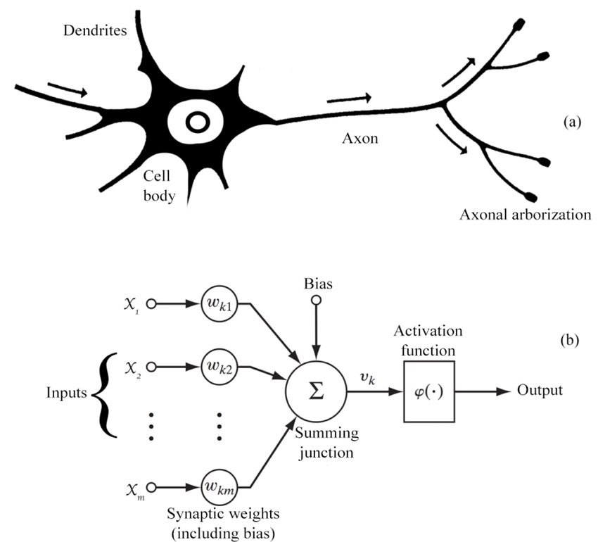
Artificial neural networks (ANNs), or connectivist systems are computing systems inspired by biological neural networks that make up the brains of animals. Such systems learn tasks (progressively improving their performance on them) by examining examples, generally without special task programming.
ANN is based on a set of connected nodes called artificial neurons (similar to biological neurons in the brain of animals). Each connection (similar to a synapse) between artificial neurons can transmit a signal from one to the other. The artificial neuron receiving the signal can process it and then signal to the artificial neurons attached to it.
In common implementations of ANNs, the signal for coupling between artificial neurons is a real number, and the output of each artificial neuron is calculated by a nonlinear function of the sum of its inputs.
Neural networks are now widespread and are used in practical tasks such as speech recognition, automatic text translation, image processing, analysis of complex processes and so on.
Fig. 1. Biological and neural networks.
Image source
What is XOR?
XOR is an exclusive or (exclusive disjunction) logical operation that outputs true only when inputs differ.
This operation can be represented as

Or by input values, XOR gives the following truth table.
| X1 | X2 | Y = X1 xor X2 |
|---|---|---|
| 0 | 0 | 0 |
| 0 | 1 | 1 |
| 1 | 0 | 1 |
| 1 | 1 | 0 |
In the book “Perceptrons: an Introduction to Computational Geometry” (published in 1969), Marvin Minsky and Seymour Papert, show that neural network with one neuron cannot solve the XOR problem.
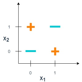
Fig. 2. How to draw one line to divide green points from red points? None.
One neuron with two inputs can form a decisive surface in the form of an arbitrary line. In order for the network to implement the XOR function specified in the table above, you need to position the line so that the four points are divided into two sets. Trying to draw such a straight line, we are convinced that this is impossible. This means that no matter what values are assigned to weights and thresholds, a single-layer neural network is unable to reproduce the relationship between input and output required to represent the XOR function.
Why use TensorFlow?
TensorFlow is an open-source machine learning library designed by Google to meet its need for systems capable of building and training neural networks and has an Apache 2.0 license.
Created by the Google Brain team, TensorFlow presents calculations in the form of stateful dataflow graphs. The library allows you to implement calculations on a wide range of hardware, from consumer devices running Android to large heterogeneous systems with multiple GPUs. TensorFlow allows you to transfer the performance of computationally intensive tasks from a single CPU environment to a heterogeneous fast environment with multiple GPUs without significant code changes TensorFlow is designed to provide massive concurrency and highly scalable machine learning for a wide range of users.
The central object of TensorFlow is a dataflow graph representing calculations. The vertices of the graph represent operations, and the edges represent tensors (multidimensional arrays that are the basis of TensorFlow). The data flow graph as a whole is a complete description of the calculations that are implemented within the session and performed on CPU or GPU devices.
Assuming you have python3 and pip3 on your computer, to install Tensorflow you need to type in the command line:
#pip3 install --user --upgrade tensorflow
Code language: CSS (css)
And to verify installation type:
#python3 -c "import tensorflow as tf; print(tf.reduce_sum(tf.random.normal([1000, 1000])))"
Code language: CSS (css)
Or type
#python3
>>>import tensorflow as tf
>>>print(tf.__version__)
1.14.0
>>>
Code language: CSS (css)
Yes, it works. Now let’s install Jupyter notebook. Jupyer notebook will help to enter code and run it in a comfortable environment.
#pip3 install jupyter
Code language: CSS (css)
And run Jupyter:
#jupyter notebook
Code language: CSS (css)
You will have a new window in your browser and will be ready to write code in Python with TensorFlow.
Additional information for installing Tensorflow on your operating system can be found here.
Basic of matrix operation
Let’s review the basic matrix operation that is required to build a neural network in TensorFlow.
C = A*B, where A and B are matrixes. The matrix A with a size of l x m and matrix B with a size m x n and result matrix C with size l x m.
Ax = b, where A is a matrix, x and b are vectors. The number of columns in A should be the same as the number of elements in vectors x and b.


Then

The classic multiplication algorithm will have complexity as O(n3).
Gradient descent
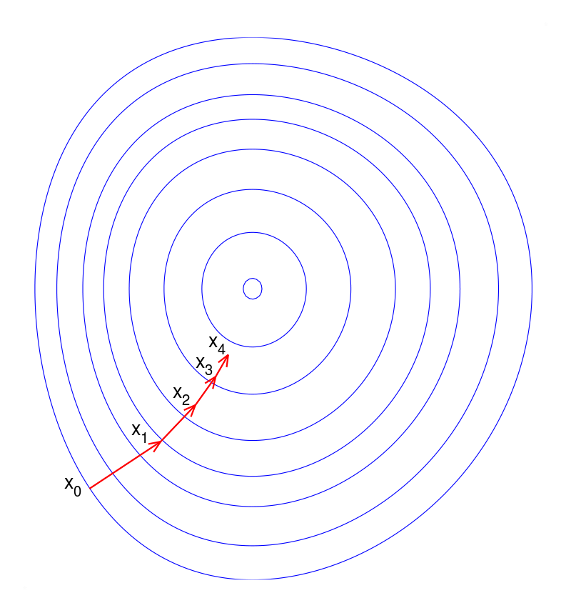
A large number of methods are used to train neural networks, and gradient descent is one of the main and important training methods. It consists of finding the gradient, or the fastest descent along the surface of the function and choosing the next solution point. An iterative gradient descent finds the value of the coefficients for the parameters of the neural network to solve a specific problem.
Gradient descent is an iterative optimization algorithm for finding the minimum of a function. To find the minimum of a function using gradient descent, we can take steps proportional to the negative of the gradient of the function from the current point.
To train the neural network, we build the error function. The error function is calculated as the difference between the output vector from the neural network with certain weights and the training output vector for the given training inputs.
If we change weights on the next step of gradient descent methods, we will minimize the difference between output on the neurons and training set of the vector. As a result, we will have the necessary values of weights and biases in the neural network and output values on the neurons will be the same as the training vector.
Gradient descent is based on the observation that if the multi-variable function F(X) is differentiable in a neighborhood of a starting point X0, then F(X) decreases fastest if one goes from point X0 in the direction of the negative gradient of -∇F(X), where ∇F(X) is a partial derivative for each variable Xi. Then we can take a step to a minimum point of function: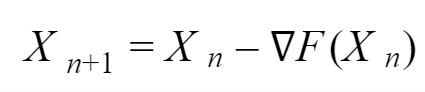
Of course, there are some other methods of finding the minimum of functions with the input vector of variables, but for the training of neural networks gradient methods work very well. They allow finding the minimum of error (or cost) function with a large number of weights and biases in a reasonable number of iterations. A drawback of the gradient descent method is the need to calculate partial derivatives for each of the input values. Very often when training neural networks, we can get to the local minimum of the function without finding an adjacent minimum with the best values. Also, gradient descent can be very slow and makes too many iterations if we are close to the local minimum.
Fig. 3. Gradient descent method.
Image source
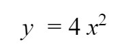
Let's look at a simple example of using gradient descent to solve an equation with a quadratic function.
import tensorflow as tf
import numpy as np

# x and y are placeholders
x = tf.placeholder(tf.float32)
y = tf.placeholder(tf.float32)

# Equation y = b*x*x
b = tf.Variable([0.0], name="b")
ys = tf.multiply(tf.multiply(x, x),b)

# Error
e = tf.square(y - ys)

# The Gradient Descent Optimizer
# 1.0 is learning_rate. The learning rate to use by Tensorflow.
train = tf.train.GradientDescentOptimizer(1.0).minimize(e)

# Create a session and run the model
model = tf.global_variables_initializer()

with tf.Session() as session:
    session.run(model)
    for i in range(50):
        x_value = np.random.rand()
        # Assume b=4, then let's find b_value = 4 and find it
  # by gradient descent
        # y = 4*x*x
        y_value = 4.0*x_value*x_value
        session.run(train, feed_dict={x: x_value, y: y_value})

    b_value = session.run(b)
    print("Predicted model: b = ", b_value)
Code language: PHP (php)
We need to find a value of a = 4 (approximately) by gradient descent. We have one variable x in this function and gradient will look like y’= 8 x and TensorFlow can calculate it automatically under the hood.
So, the answer is equal to 3.9999995 with 100 iterations on TensorFlow gradient descent. If we will make more than 50 iterations, the result will be more accurate.
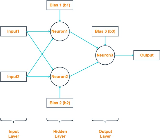
Building and training XOR neural network
Now let's build the simplest neural network with three neurons to solve the XOR problem and train it using gradient descent.
If we imagine such a neural network in the form of matrix-vector operations, then we get this formula.
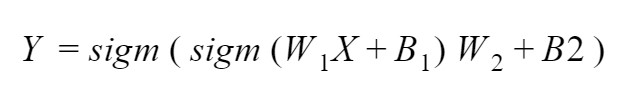
Where:
- X is an input value vector, size 2x1 elements
- W1 is a matrix of the coefficient for the first layer, size 2x2 elements
- B1 is a bias for the first layer, a vector with 2x1 elements
- W2 is a vector of the coefficient for the first layer, size 2x1 elements
- B2 is a value of bias for the second layer, size 1x1 element
- Y is an output value, size 1x1 element
- sigm(x) is a sigmoid activation function for neural network
# coding=utf-8
import tensorflow as tf
print (tf.VERSION)

# input X vector
X = [[0, 0], [0, 1], [1, 0], [1, 1]]
# output Y vector
Y = [[0], [1], [1], [0]]

# Placeholders for input and output
x = tf.placeholder(tf.float32, shape=[4,2])
y = tf.placeholder(tf.float32, shape=[4,1])

# W matrix
W1 = tf.Variable([[1.0, 0.0], [1.0, 0.0]], shape=[2,2])
W2 = tf.Variable([[0.0], [1.0]], shape=[2,1])

# Biases
B1 = tf.Variable([0.0, 0.0], shape=[2])
B2 = tf.Variable([0.0], shape=1)

# Hidden layer and outout layer
output =tf.sigmoid(tf.matmul(tf.sigmoid(tf.matmul(x, W1) + B1), W2) + B2)

# error estimation
e = tf.reduce_mean(tf.squared_difference(y, output))
train = tf.train.GradientDescentOptimizer(0.1).minimize(e)

init = tf.global_variables_initializer()
sess = tf.Session()
sess.run(init)

for i in range (100001):
    error = sess.run(train, feed_dict={x: X, y: Y})
    if i % 10000 == 0:
        print('\nEpoch: ' + str(i))
        print('\nError: ' + str(sess.run(e, feed_dict={x: X, y: Y})))
        for el in sess.run(output, feed_dict={x: X, y: Y}):
            print('    ',el)
sess.close()

print ("Complete")
Code language: PHP (php)
Test the solution
And now let's run all this code, which will train the neural network and calculate the error between the actual values of the XOR function and the received data after the neural network is running. The closer the resulting value is to 0 and 1, the more accurately the neural network solves the problem.
1.14.0

Epoch: 0
Error: 0.26442584
     [0.6202572]
     [0.6200183]
     [0.6200183]
     [0.6198486]

Epoch: 10000
Error: 0.07002328
     [0.20779318]
     [0.7534747]
     [0.7534747]
     [0.33965528]

...

Epoch: 100000
Error: 0.0005582984
     [0.02478384]
     [0.9782787]
     [0.9782787]
     [0.02598701]
Complete
Code language: CSS (css)
And so we see that for 100,000 iterations we got an error of 0.0005582984 and the output values are close to 0 and 1. That is, the neural network coped with its task.
Using different optimizer
Now let's change one line in the code. Replace the gradient descent with the Adam optimizer.
train = tf.train.AdamOptimizer(0.1).minimize(e)
And we will have a significantly better result. When using Adam's optimizer, we get the result of a neural network in just 1000 iterations and with error 8.665349e-05.
1.14.0

Epoch: 0

Error: 0.25394842
     [0.56893826]
     [0.5577527]
     [0.5577527]
     [0.54857785]
Epoch: 100

...

Epoch: 1000

Error: 8.665349e-05
     [0.00908105]
     [0.99136895]
     [0.99136895]
     [0.01073119]
Complete
Code language: CSS (css)
Adam’s optimizer was presented by Diederik Kingma from OpenAI and Jimmy Ba from the University of Toronto in their 2015 ICLR paper ”Adam: A Method for Stochastic Optimization”. Adam is an algorithm that is a first-order method based on adaptive estimates of lower-order moments. This method implements the benefits of two other methods AdaGrad and RMSProp. The algorithm calculates an exponential moving average of the gradient and the squared gradient. It is highly recommended for training deep learning networks.
Conclusion
And so, what we did get as a result? It turns out that TensorFlow is quite simple to install and matrix calculations can be easily described on it. The beauty of this approach is the use of a ready-made method for training a neural network. The article provides a separate piece of TensorFlow code that shows the operation of the gradient descent. This facilitates the task of understanding neural network training. A slightly unexpected result is obtained using gradient descent since it took 100,000 iterations, but Adam's optimizer copes with this task with 1000 iterations and gets a more accurate result.
We wish you successful projects with TensorFlow.