Python libraries math, scipy, numpy, matplotlib

There is such a thing as Python programming language. It is valuable in itself for a number of reasons, as it is effective and very common. In addition to everything else, Python is valuable for its set of libraries for a variety of needs.

The fields of mathematical calculations, computer modeling, economic calculations, machine learning, statistics, engineering, and other industries are widely used by a number of Python libraries, some of which we will consider in this article.

These libraries save developers time and standardize work with mathematical functions and algorithms, which puts Python code writing for many industries at a very high level.

Let's look at these libraries in order and determine which sections of development they are responsible for and how they are interconnected.

Math

To carry out calculations with real numbers, the Python language contains many additional functions collected in a library (module) called math.

To use these functions at the beginning of the program, you need to connect the math library, which is done by the command 

import math

Python provides various operators for performing basic calculations, such as * for multiplication,% for a module, and / for the division. If you are developing a program in Python to perform certain tasks, you need to work with trigonometric functions, as well as complex numbers. Although you cannot use these functions directly, you can access them by turning on the math module math, which gives access to hyperbolic, trigonometric and logarithmic functions for real numbers. To use complex numbers, you can use the math module cmath. When comparing math vs numpy, a math library is more lightweight and can be used for extensive computation as well.

The Python Math Library is the foundation for the rest of the math libraries that are written on top of its functionality and functions defined by the C standard. Please refer to the python math examples for more information.

Number-theoretic and representation functions

This part of the mathematical library is designed to work with numbers and their representations. It allows you to effectively carry out the necessary transformations with support for NaN (not a number) and infinity and is one of the most important sections of the Python math library. Below is a short list of features for Python 3rd version. A more detailed description can be found in the documentation for the math library.

• math.ceil(x) - return the ceiling of x, the smallest integer greater than or equal to x
• math.comb(n, k) - return the number of ways to choose k items from n items without repetition and without order
• math.copysign(x, y) - return float with the magnitude (absolute value) of x but the sign of y. On platforms that support signed zeros, copysign (1.0, -0.0) returns -1.0
• math.fabs(x) - return the absolute value of x
• math.factorial(x) - return x factorial as an integer. Raises ValueError if x is not integral or is negative
• math.floor(x) - return the floor of x, the largest integer less than or equal to x
• math.fmod(x, y) - return fmod(x, y), as defined by the platform C library
• math.frexp(x) - return the mantissa and exponent of x as the pair (m, e). m is a float and e is an integer such that x == m * 2**e exactly
• math.fsum(iterable) - return an accurate floating-point sum of values in the iterable
• math.gcd(a, b) - return the greatest common divisor of the integers a and b
• math.isclose(a, b, *, rel_tol=1e-09, abs_tol=0.0) - return True if the values a and b are close to each other and False otherwise
• math.isfinite(x) - return True if x is neither infinity nor a NaN, and False otherwise (note that 0.0 is considered finite)
• math.isinf(x) - return True if x is positive or negative infinity, and False otherwise
• math.isnan(x) - return True if x is a NaN (not a number), and False otherwise
• math.isqrt(n) - return the integer square root of the nonnegative integer n. This is the floor of the exact square root of n, or equivalently the greatest integer a such that a² ≤ n
• math.ldexp(x, i) - return x * (2**i). This is essentially the inverse of function frexp()
• math.modf(x) - return the fractional and integer parts of x. Both results carry the sign of x and are floats
• math.perm(n, k=None) - return the number of ways to choose k items from n items without repetition and with order
• math.prod(iterable, *, start=1) - calculate the product of all the elements in the input iterable. The default start value for the product is 1
• math.remainder(x, y) - return the IEEE 754-style remainder of x with respect to y
• math.trunc(x) - return the Real value x truncated to an Integral (usually an integer)

Power and logarithmic functions

The power and logarithmic functions section are responsible for exponential calculations, which is important in many areas of mathematics, engineering, and statistics. These functions can work with both natural logarithmic and exponential functions, logarithms modulo two, and arbitrary bases.

• math.exp(x) - return e raised to the power x, where e = 2.718281… is the base of natural logarithms
• math.expm1(x) - return e raised to the power x, minus 1. Here e is the base of natural logarithms. math.log(x[, base]) - With one argument, return the natural logarithm of x (to base e). With two arguments, return the logarithm of x to the given base, calculated as log(x)/log(base)
• math.log1p(x) - return the natural logarithm of 1+x (base e). The result is calculated in a way that is accurate for x near zero
• math.log2(x) - return the base-2 logarithm of x. This is usually more accurate than log(x, 2)
• math.log10(x) - return the base-10 logarithm of x. This is usually more accurate than log(x, 10)
• math.pow(x, y) - return x raised to the power y
• math.sqrt(x) - return the square root of x

Trigonometric functions

Trigonometric functions, direct and inverse, are widely represented in the Python Mathematical Library. They work with radian values, which is important. It is also possible to carry out calculations with Euclidean functions.

• math.acos(x) - return the arc cosine of x, in radians
• math.asin(x) - return the arc sine of x, in radians
• math.atan(x) - return the arctangent of x, in radians
• math.atan2(y, x) - return atan(y / x), in radians. The result is between -pi and pi
• math.cos(x) - return the cosine of x radians
• math.dist(p, q) - return the Euclidean distance between two points p and q, each given as a sequence (or iterable) of coordinates. The two points must have the same dimension
• math.hypot(*coordinates) - return the Euclidean norm, sqrt(sum(x**2 for x in coordinates)). This is the length of the vector from the origin to the point given by the coordinates
• math.sin(x) - return the sine of x radians
• math.tan(x) - return the tangent of x radians

Angular conversion

Converting degrees to radians and vice versa is a fairly common function and therefore the developers have taken these actions to the Python library. This allows you to write compact and understandable code.

• math.degrees(x) - convert angle x from radians to degrees
• math.radians(x) - convert angle x from degrees to radians

Hyperbolic functions

Hyperbolic functions are analogs of trigonometric functions that are based on hyperbolas instead of circles.

• math.acosh(x) - return the inverse hyperbolic cosine of x
• math.asinh(x) - return the inverse hyperbolic sine of x
• math.atanh(x) - return the inverse hyperbolic tangent of x
• math.cosh(x) - return the hyperbolic cosine of x
• math.sinh(x) - return the hyperbolic sine of x
• math.tanh(x) - return the hyperbolic tangent of x

Special functions

The special functions section is responsible for error handling and gamma functions. This is a necessary function and it was decided to implement it in the standard Python mathematical library.

• math.erf(x) - Return the error function at x
• math.erfc(x) - Return the complementary error function at x
• math.gamma(x) - Return the Gamma function at x
• math.lgamma(x) - Return the natural logarithm of the absolute value of the Gamma function at x

Constants

The constant section provides ready-made values for basic constants and writes them with the necessary accuracy for a given hardware platform, which is important for Python's portability as a cross-platform language. Also, the very important values infinity and “not a number” are defined in this section of the Python library.

• math.pi - the mathematical constant π = 3.141592…, to available precision
• math.e - the mathematical constant e = 2.718281…, to available precision
• math.tau - the mathematical constant τ = 6.283185…, to available precision. Tau is a circle constant equal to 2π, the ratio of a circle’s circumference to its radius
• math.inf - a floating-point positive infinity. (For negative infinity, use -math.inf.) Equivalent to the output of float('inf')
• math.nan - a floating-point “not a number” (NaN) value. Equivalent to the output of float('nan')

Scipy

SciPy is a library for the open-source Python programming language, designed to perform scientific and engineering calculations.

The capabilities of this library are quite wide:

• Search for minima and maxima of functions
• Calculation of function integrals
• Support for special functions
• Signal processing
• Image processing
• Work with genetic algorithms
• Solving ordinary differential equations

SciPy in Python is a collection of mathematical algorithms and functions built as a Numpy extension. It greatly extends the capabilities of an interactive Python session by providing the user with high-level commands and classes for managing and visualizing data. With SciPy, an interactive Python session becomes a data processing and prototyping system competing with systems such as MATLAB, IDL, Octave, R-Lab, and SciLab.

An additional advantage of Python-based SciPy is that it is also a fairly powerful programming language used in the development of complex programs and specialized applications. Scientific applications also benefit from the development of additional modules in numerous software niches by developers around the world. Everything from parallel programming for the web to routines and database classes is available to the Python programmer. All of these features are available in addition to the SciPy math library.
Packages for mathematical methods

SciPy is organized into sub-packages covering various scientific computing areas:

• cluster - Clustering Algorithms
• constants - physical and mathematical constants
• fftpack - Fast Fourier Transform subroutines
• integrate - integration and solution of ordinary differential equations
• Interpolate - interpolation and smoothing splines
• io - input and output
• linalg - linear algebra
• ndimage - n-dimensional image processing
• odr -orthogonal regression distance multiplexing
• optimize - root structure optimization and search
• signal - signal processing
• sparse - sparse matrices and related procedures
• spatial - spatial Data Structures and Algorithms
• special - special functions
• stats - statistical Distributions and Functions
• weave - C / C ++ integration

The SciPy ecosystem includes general and specialized tools for data management and computation, productive experimentation, and high-performance computing. Below, we overview some key packages, though there are many more relevant packages.

Main components of ScyPy

Data and computation:

• pandas, providing high-performance, easy-to-use data structures
• SymPy, for symbolic mathematics and computer algebra
• scikit-image is a collection of algorithms for image processing
• scikit-learn is a collection of algorithms and tools for machine learning
• h5py and PyTables can both access data stored in the HDF5 format

Productivity and high-performance computing:

• IPython, a rich interactive interface, letting you quickly process data and test ideas
• The Jupyter notebook provides IPython functionality and more in your web browser, allowing you to document your computation in an easily reproducible form
• Cython extends Python syntax so that you can conveniently build C extensions, either to speed up critical code or to integrate with C/C++ libraries
• Dask, Joblib or IPyParallel for distributed processing with a focus on numeric data

Quality assurance:

• nose, a framework for testing Python code, being phased out in preference for pytest
• numpydoc, a standard, and library for documenting Scientific Python libraries

SciPy provides a very wide and sought-after feature set:

• Clustering package (scipy.cluster)
• Constants (scipy.constants)
• Discrete Fourier transforms (scipy.fftpack)
• Integration and ODEs (scipy.integrate)
• Interpolation (scipy.interpolate)
• Input and output (scipy.io)
• Linear algebra (scipy.linalg)
• Miscellaneous routines (scipy.misc)
• Multi-dimensional image processing (scipy.ndimage)
• Orthogonal distance regression (scipy.odr)
• Optimization and Root Finding (scipy.optimize)
• Signal processing (scipy.signal)
• Sparse matrices (scipy.sparse)
• Sparse linear algebra (scipy.sparse.linalg)
• Compressed Sparse Graph Routines (scipy.sparse.csgraph)
• Spatial algorithms and data structures (scipy.spatial)
• Special functions (scipy.special)
• Statistical functions (scipy.stats)
• Statistical functions for masked arrays (scipy.stats.mstats)
• Low-level callback functions

An example of how to calculate effectively on SciPy

In this tutorial, Basic functions — SciPy v1.4.1 Reference Guide, you can find how to calculate polynomials, their derivatives, and integrals. Yes, by one line of code SciPy calculates derivative and integral in symbolic form. Imagine how many lines of code you would need to do this without SciPy. This is why this library is valuable in Python:

>>> p = poly1d([3,4,5])
>>> print(p)
   2
3 x + 4 x + 5
>>> print(p*p)
   4      3      2
9 x + 24 x + 46 x + 40 x + 25
>>> print(p.integ(k=6))
   3     2
1 x + 2 x + 5 x + 6
>>> print(p.deriv())
6 x + 4
>>> p([4, 5])
array([ 69, 100])

Numpy

In early 2005, programmer and data scientist Travis Oliphant wanted to unite the community around one project and created the NumPy library to replace the Numeric and NumArray libraries. NumPy was created based on the Numeric code. The Numeric code was rewritten to be easier to maintain, and new features could be added to the library. NumArray features have been added to NumPy.

NumPy was originally part of the SciPy library. To allow other projects to use the NumPy library, its code was placed in a separate package.

The source code for NumPy is publicly available. NumPy is licensed under the BSD license.

Purpose of the NumPy library

Mathematical algorithms implemented in interpreted languages, for example, Python, often work much slower than the same algorithms implemented in compiled languages (for example, Fortran, C, and Java). The NumPy library provides implementations of computational algorithms in the form of functions and operators, optimized for working with multidimensional arrays. As a result, any algorithm that can be expressed as a sequence of operations on arrays (matrices) and implemented using NumPy works as fast as the equivalent code executed in MATLAB. If we compare numpy vs math, we quickly find thatnumpy has more advantages for computation methods compared to math.

Here are some of the features of Numpy:

• A powerful N-dimensional array object
• Sophisticated (broadcasting) functions
• Tools for integrating C/C++ and Fortran code
• Useful linear algebra, Fourier transform, and random number capabilities

What’s the difference between a Python list and a NumPy array?

As described in the NumPy documentation, “NumPy gives you an enormous range of fast and efficient ways of creating arrays and manipulating numerical data inside them. While a Python list can contain different data types within a single list, all of the elements in a NumPy array should be homogenous. The mathematical operations that are meant to be performed on arrays would be extremely inefficient if the arrays weren’t homogenous.”

NymPy User Features

Numpy provides the following features to the user:

• Array objects
• Constants
• Universal functions (ufunc)
• Routine
• Packaging (numpy.distutils)
• NumPy Distutils - Users Guide
• NumPy C-API
• NumPy internals
• NumPy and SWIG

NumPy basics:

• Data types
• Array creation
• I/O with NumPy
• Indexing
• Broadcasting
• Byte-swapping
• Structured arrays
• Writing custom array containers
• Subclassing ndarray

One of the main objects of NumPy is ndarray. It allows you to create multidimensional data arrays of the same type and perform operations on them with great speed. Unlike sequences in Python, arrays in NumPy have a fixed size, the elements of the array must be of the same type. You can apply various mathematical operations to arrays, which are performed more efficiently than for Python sequences.

The next example shows how to work with linear algebra with NumPy. It is really simple and easy-to-understand for Python users.

>>> import numpy as np
>>> a = np.array([[1.0, 2.0], [3.0, 4.0]])
>>> print(a)
[[ 1.  2.]
 [ 3.  4.]]

>>> a.transpose()
array([[ 1.,  3.],
       [ 2.,  4.]])

>>> np.linalg.inv(a)
array([[-2. ,  1. ],
       [ 1.5, -0.5]])

>>> u = np.eye(2) # unit 2x2 matrix; "eye" represents "I"
>>> u
array([[ 1.,  0.],
       [ 0.,  1.]])
>>> j = np.array([[0.0, -1.0], [1.0, 0.0]])

>>> j @ j        # matrix product
array([[-1.,  0.],
       [ 0., -1.]])

>>> np.trace(u)  # trace
2.0

>>> y = np.array([[5.], [7.]])
>>> np.linalg.solve(a, y)
array([[-3.],
       [ 4.]])

>>> np.linalg.eig(j)
(array([ 0.+1.j,  0.-1.j]), array([[ 0.70710678+0.j,0.70710678-0.j],
       [ 0.00000000-0.70710678j,  0.00000000+0.70710678j]]))

Numpy allows processing information without cycles. Please take a look at this article published by Brad Solomon about the advantages of Numpy: “It is sometimes said that Python, compared to low-level languages such as C++, improves development time at the expense of runtime. Fortunately, there are a handful of ways to speed up operation runtime in Python without sacrificing ease of use. One option suited for fast numerical operations is NumPy, which deservedly bills itself as the fundamental package for scientific computing with Python.” It makes computation in Python really fast. 

Matplotlib

Neuroscientist John D. Hunter began developing matplotlib in 2003, mainly inspired by the emulation of Mathworks MATLAB software teams. Matplotlib is today a whole product of the community: it is developed and supported by many people. John talked about the evolution of matplotlib at the SciPy conference in 2012.

Learning matplotlib at times can be a difficult process. The problem is not the lack of documentation (which is very extensive, by the way). Difficulties may arise with the following:

• The size of the library is huge in itself, about 70,000 lines of code
• Matplotlib contains several different interfaces (ways to build a figure) and can interact with a large number of backends. (The backends are responsible for how in fact the diagrams will be displayed, not only for the internal structure)
• Despite the vastness, some of the matplotlib's own documentation is seriously outdated. The library is still evolving, and many old examples on the web may include 70% less code than in their current version

Understanding that matplotlib roots grow from MATLAB helps explain the existence of pylab. pylab is a module inside the matplotlib library that has been built in to emulate the overall MATLAB style. It exists only for introducing a number of class functions from NumPy and matplotlib into the namespace, which simplifies the transition of MATLAB users who did not encounter the need for import statements. Former MATLAB users love its functionality, because with from pylab import * they can simply call plot() or array() directly, just like they did in MATLAB.

Key features of Matplotlib

One of the business cards of matplotlib is the hierarchy of its objects. If you have already worked with the matplotlib introductory manual, you may have already called something like plt.plot ([1, 2, 3]). This one line indicates that the graph is actually a hierarchy of Python objects. By “hierarchy” we mean that each chart is based on a tree-like structure of matplotlib objects.

The Figure object is the most important external container for matplotlib graphics, which can include several Axes objects. The reason for the difficulty in understanding may be the name: Axes (axes), in fact, turn into what we mean by an individual graph or chart (rather than the plural “axis”, as you might expect).

You can think of the Figure object as a box-like container containing one or more Axes objects (real graphs). Below Axes objects, in a hierarchical order, are smaller objects such as individual lines, elevations, legends, and text boxes. Almost every “element” of a diagram is its own manipulated Python object, right up to labels and markers. An example chart on the matplot is located below.
Image source

Matplotlib is a flexible, easily configurable package that, along with NumPy, SciPy, and IPython, provides features similar to MATLAB. The package currently works with several graphics libraries, including wxWindows and PyGTK.

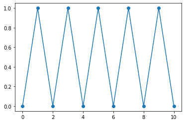
Python code example for plotting

The Python code itself is quite simple and straightforward. Here's an example of a simple plot:

import matplotlib.pyplot as plt 

x = [0,1,2,3,4,5,6,7,8,9,10]
y = [0,1,0,1,0,1,0,1,0,1,0] 
plt.plot(x, y, marker="o")
plt.show()

Types of graphs and charts

The package supports many types of graphs and charts:

• Charts (line plot)
• Scatter plot
• Bar charts and histograms
• Pie Chart
• Chart trunk (stem plot)
• Contour plots
• Gradient Fields (quiver)
• Spectrograms
• The user can specify the coordinate axis, grid, add labels and explanations, use a logarithmic scale or polar coordinates

Image source

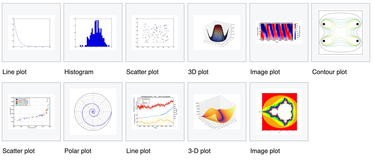
Simple 3D graphics can be built using the mplot3d toolkit. There are other toolkits: for mapping, for working with Excel, utilities for GTK and others. With Matplotlib, you can make animated images.

Matplotlib can be technically and syntactically complex. To create a ready-made diagram, it can take half an hour to google search alone and combine all this hash to fine-tune the graph. However, understanding how matplotlib interfaces interact with each other is an investment that can pay off. 

Conclusion

In conclusion, the Python 3 math module, along with numpy, scipy, and matplotlib libraries, give Python users exactly the capabilities that we really need in real projects in economics, engineering calculations, mathematics, forecasting, computer modeling, and big data processinga. Importantly, these libraries combine very well with each other; you can build graphs from numpy using matplot, use numpy objects, call the necessary scipy methods. If you look at the problem closely, then the need to write your own methods has already disappeared, except for some special functions and algorithms. If you need to implement a specific project in this area, you can contact Svitla Systems, where qualified developers and testers will carry out the implementation of your task and ensure its reliable support.