Time Series Forecasting Based on AutoRegression

It is often necessary to quickly and efficiently calculate time series values to assess the behavior of an observed object or process. This can be an indicator of the company's performance in a certain direction, the temperature inside the room, the cost of a certain product for a promotion, an assessment of customer satisfaction with service, and so on.

Practical problems of this class have to be solved quite often, and instead of building the expected curve using a spreadsheet editor or pencil and paper, you can quickly and efficiently use Python and the Google Colab cloud service. We will choose the simplest and most popular method, autoregressive (AR), as a method for forecasting a time series.

Let's see how to solve this problem using the example of data on Covid-19 in Ukraine, specifically the number of new cases detected daily.

Time Series

A time series (or a dynamic series) is statistical material collected at different points in time about the value of any parameters (in the simplest case, one) of the process under study. Each unit of statistical material is called a measurement or data sample at a specific moment in time.

The time series for each sample must indicate the measurement time or the number of measurements in order. A time series differs significantly from a simple data sample since the analysis takes into account the relationship of measurements to time, and not only the statistical diversity and statistical characteristics of the sample.

A time series consists of two elements:

• the period of time for which or as of which the numerical values are given;
• numerical values of one or another indicator called the levels of the series.

A time series can be classified by the number of indicators for which the levels are determined at each point in time: one-dimensional and multi-dimensional time series.

Also, time series are divided depending on the presence of the main trend, while stationary series, in which the main value and variance are constant, and non-stationary ones, containing the main development trend, are distinguished.

Why use forecasting methods in data science?

A time series is one of the most important forecasting methods in various fields of human activity and natural phenomena. Time series, as a rule, results from the measurement of some indicator. These can be both indicators (characteristics) of technical systems, and indicators of natural, social, economic, and other systems, for example, weather data. A typical example of a time series is the stock exchange rate, for which the purpose is to determine the main direction of development or trends.

Currently, there are about 220 forecasting methods, but most often no more than 10 are used in practice.  These include: factual (extrapolation, interpolation, trend analysis), expert (including survey, questionnaire), the publication (including patent), citation-index, scenario, matrix, modeling, analogies, and building graphs.

Forecast estimates using extrapolation methods are calculated in several stages:

• forecast baseline check
• identification of patterns of the past development of the phenomenon
• assessment of the degree of reliability of the revealed pattern of development in the past (selection of the trend function)
• extrapolation - transferring the identified patterns to a certain period of the future
• correction of the obtained forecast, taking into account the results of a meaningful analysis of the current state.

To obtain an objective forecast of the development of the phenomenon under study, the baseline data must meet the following requirements:

• the time step for the entire baseline must be the same
• observations are recorded at the same moment of every time interval (for example, at noon of every day, the first of every month)
• the baseline must be complete, that is, no data skipping is allowed.

If there are no results in the observations for a short period of time, then to ensure the completeness of the baseline, it is necessary to fill them in with approximate data. For example, use the average value of adjacent segments.

Correction of the obtained forecast is performed to clarify the obtained long-term forecasts, taking into account the influence of seasonality or abrupt development of the phenomenon under study.

When predicting an object, you often have to predict not one, but several of its indicators. In this case, the forecast of the development of one indicator can be performed by one method, and another indicator by another method, i.e., combinations of methods are used.

The most popular methods in time series forecasting are:

• Autoregression (AR)
• Moving Average (MA)
• Autoregressive Moving Average (ARMA)
• Autoregressive Integrated Moving Average (ARIMA)
• Seasonal Autoregressive Integrated Moving-Average (SARIMA)
• Seasonal Autoregressive Integrated Moving-Average with Exogenous Regressors (SARIMAX)
• Vector Autoregression (VAR)
• Vector Autoregression Moving-Average (VARMA)
• Vector Autoregression Moving-Average with Exogenous Regressors (VARMAX)
• Simple Exponential Smoothing (SES)
• Holt Winter’s Exponential Smoothing (HWES)

All these methods can be used in time series forecasting, but some methods will be more effective in specific areas of domains. In practice, a  combination of methods will generate better results.

How to make simple and effective time series forecasting on AutoRegression model

In statistics, economics, and digital signal processing, an autoregressive (AR) model, a random process, is common. It is used to describe certain time-varying processes in nature, sociology, economics, electronic and mechanical systems, and many other fields.

The autoregressive model determines that the output variable is linearly dependent on its own previous values and on the stochastic term (responsible for a parameter that cannot be fully predicted). The model takes the form of a stochastic difference equation (or a recurrence relation, but not in the form of a differential equation).

Together with the moving average (MA) model, it is a special case and a key component of the more general autoregressive moving average (ARMA) and autoregressive integrated moving average (ARIMA) time series models.

The AR model of the time series, in general, is described as a formula: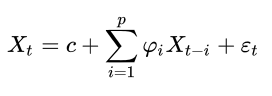

Where are the model parameters and et are the white noise values. Where p is the number of values by which the dependency is determined (aka lags).

For practical use of AR, the method is easiest to run in Python: for this, you can download the ready-made statsmodel library. You can read more about this library here.

As a practical and relevant task, we will choose the time series of the daily parameter of the detected new cases of COVID-19 in Ukraine (according to official sources).

In order to run a real example AR method, go to Google Colab and start by installing the statsmodel package, which can be easily done via pip install.

%pip install statsmodels --upgrade

After that, do not forget to restart the runtime. Without this, it will not work, since the environment does not see the newly installed package. To restart, click on the “RESTART RUNTIME” button.

Let's train the model using AutoReg() and then predict using model_fit.predict() for the future 21 values (we predict three weeks ahead).

Set the lags parameter to 7, since the nature of the input data has a weekly frequency.

from statsmodels.tsa.ar_model import AutoReg
from random import random
# contrived dataset
data = numpy.array([4,7,2,10,21,26,11,29,83,22,92,46,119,73,97,149,
148,154,155,68,143,206,224,311,308,266,325,270,392,397,501,444,343,261,415,
467,578,477,478,492,392,401,456,540,455,550,502,418,366,487,507,504,515,522,
416,375,402,422,483,528,433,325,260,354,476,442,432,406,259,339,321,477,
429,393,468,340,328,482,589,553,550,485,463,394,525,689,683,753,648,656,
666,758,829,921,841,735,681,833,940,994,1109,948,917,646,706,664,889,876,
914,823,543,564,807,810,819,800,678,612,638,836,848,809,847,731,651,673,
829,856,972,1106,920,807,919,1022,1197,1090,1172,1112,990,1061,1271,1318,
1453,1489,1199,1008,1158,1433,1592,1732,1847,1637,1464,1616,1967,2134,2106,
2328,1987,1799,1658,1670,1974,2438,2481,2096,2141,2088,2495,2430,2723,2836,
2107,2174,2411,2551,2582,3144,3103,2476,2462,2905])
 
# fit model
model = AutoReg(data, lags=7)
model_fit = model.fit()
# let's make prediction
y = model_fit.predict(len(data), len(data)+21)
print(y)

plt.figure(figsize=(10,5))
plt.plot(range(1,len(y)+1), y, 'b')
plt.show()

Then we get a forecast graph for 21 days according to the previous values.

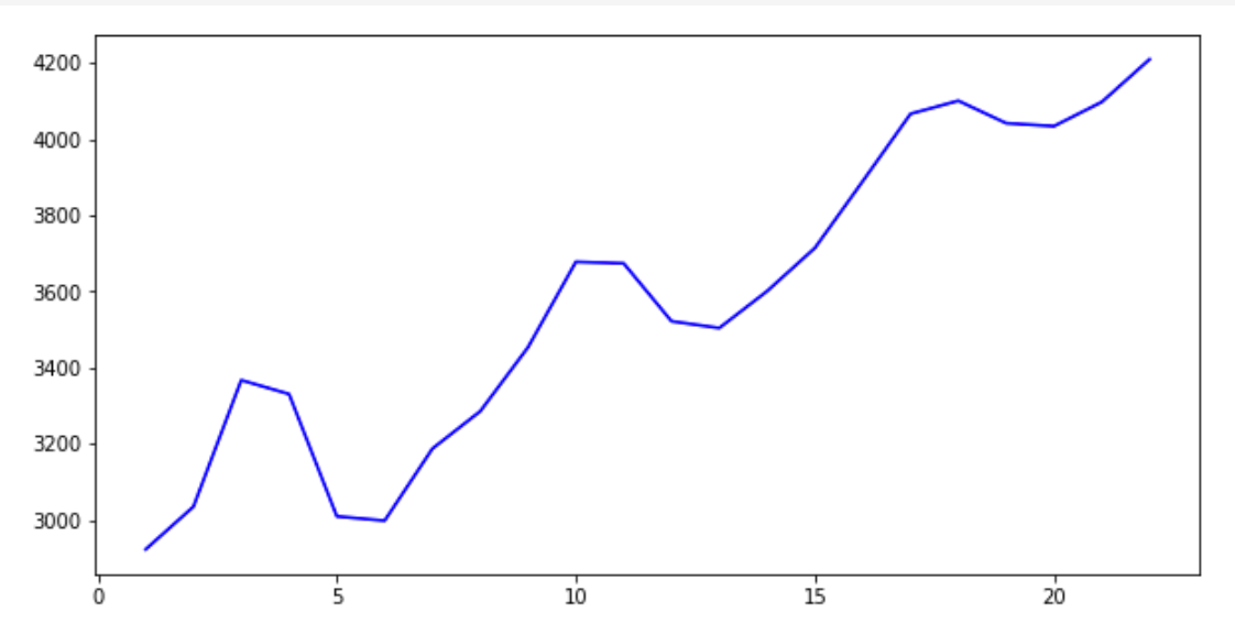
But in this form, it is very difficult to visually assess how this graph is combined with the previous values. Therefore, let's add the old values (blue graph) and new values (red graph) in one picture.

plt.figure(figsize=(10,5))
prognose = numpy.concatenate((data,y))
plt.plot(range(1,len(prognose)+1), prognose, 'r')
plt.plot(range(1,len(data)+1), data, 'b')
plt.show()

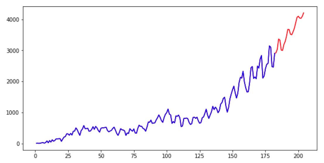
Now let's change the value of lags = 75 to increase the impact of more data in the window, and see how the predicted value changes.

# fit model
model = AutoReg(data, lags=75)
model_fit = model.fit()
# make prediction
y = model_fit.predict(len(data), len(data)+20)
print(y)
 
plt.figure(figsize=(10,5))
prognose = numpy.concatenate((data,y))
plt.plot(range(1,len(prognose)+1), prognose, 'r')
plt.plot(range(1,len(data)+1), data, 'b')
plt.show()

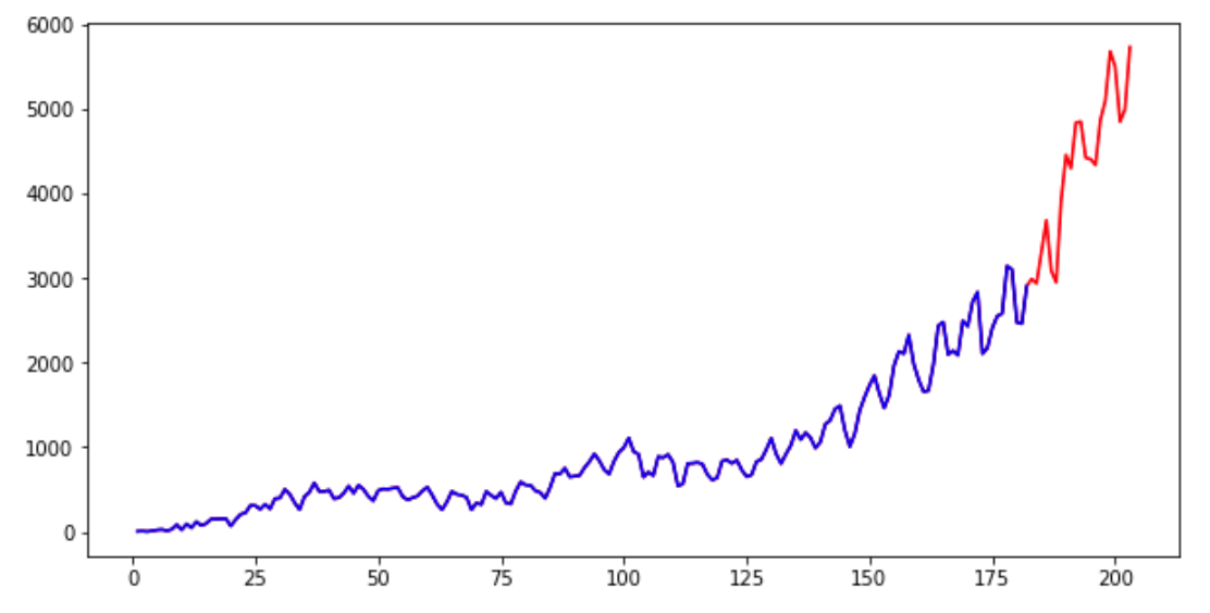
As you can see, taking into account a larger number of previous values, we get a decent increase in the absolute values of the predicted parameter. Both results are plausible though.

Conclusion

If you are interested in the topic of time series and like the idea of using these methods in practice, we strongly recommend reading about other methods in the article by Dr. Jason Brownlee (Ph.D.) at this link.

There you will find descriptions of more advanced methods and can expand your toolbox specifically for your task.

Our experts from Svitla Systems will assist you in the research and development of machine learning and data analysis methods. Since the education system in our main locations prepares engineers who are savvy in mathematics and programming, you can contact our company for solving a problem even if you cannot clearly formulate it, but need a solution for your business process.

Our system analysts and experienced project managers will assess the project at a high level, will talk with you to clarify the tasks for the project, and choose the right development toolkit. At the same time, the copyrights are fully and completely retained by your company. Svitla Systems operates in many locations on several continents and will always find the right team for you to solve your software development and data science tasks.