Linear Optimization with Python

Mathematical studies of individual economic problems and mathematical formalization of numerical data was carried out as far back as the 19th century. In mathematical analysis of the extended production process, algebraic relations were used. Their analysis was carried out using differential calculus. Linear programming is a mathematical method that is used to determine the best possible result or solution from a given set of parameters or a list of requirements. These requirements can be represented in the form of linear relationships. Most often, linear programming is used in computer modeling or simulation to find the best solution in the distribution of finite resources, such as money, energy, labor, machine resources, time, space, and many other values. As often happens, the “best result” required for linear programming in practice is maximum profit or minimum cost. Linear programming is used as a mathematical method to determine and plan the best results. The method was developed by Leonid Kantorovich in 1937. This was the method used to plan expenses and revenues in such a way as to reduce costs for military projects.

What is Linear Programming

A general or standard linear programming problem is the problem of finding the minimum of a linear objective function in linear form as: The problem in which inequality constraints appear is called the main linear programming problem: Linear programming problems of the most general form (problems with mixed constraints: equalities and inequalities, the presence of variables that are free from constraints) can be reduced to equivalent (having the same set of solutions) substitutions of variables and replacing equalities with a pair of inequalities. The problem of finding the maximum can be replaced by the problem of finding the minimum by taking the coefficients c with the opposite sign.

Python library for Linear Programming

There are many implementations of  linear programming Python libraries. Most valuables of them are:

• PuLP and/or Pyomo. PuLP is an LP modeler written in Python. Pyomo is a Python-based, open-source optimization modeling language with a diverse set of optimization capabilities.
• CVXOPT is written by Lieven Vandenberghe and some of his collaborators. CVXOPT is a free software package for convex optimization based on the Python programming language.
• Or-tools Google's software suite for combinatorial optimization. This is an open-source, fast, and portable software suite for solving combinatorial optimization problems.
• Scipy.optimize.linprog The SciPy linear programming library minimizes a linear objective function subject to linear equality and inequality constraints.

Transport task

There is some uniform cargo that needs to be transported from n warehouses to m plants. For each warehouse i it is known how much cargo ai is in it, and for each plant its need bj for cargo is known. The transportation cost is proportional to the distance from the warehouse to the plant (all distances cij from the i-th warehouse to the j-th plant are known). It is required to create the cheapest transportation plan. The decisive variables, in this case, are xij - the amount of cargo transported from the i-th warehouse to the j-th plant. They satisfy the restrictions: The objective function has the form: which must be minimized. Then we will have a minimum value of budget constraint for transportation from warehouses to plants.

Example of Linear Programming Problem

We solve the following transportation problem. To get started, take the simplest linprog Python example to figure out how scipy.optimize.linprog() works. Consider the following problem. There are 2 warehouses and 1 plant. Raw materials are transported from warehouses to the plant. The first warehouse has a1 = 4 tons of raw materials. The second warehouse has a2 = 6 tons of raw materials. The plant has a need for b = 8 tons of raw materials. The cost of transportation from the first warehouse c1 = 1 thousand dollars. The cost of transportation from the second warehouse c2 = 1.5 thousand dollars. 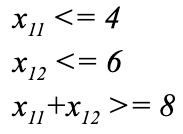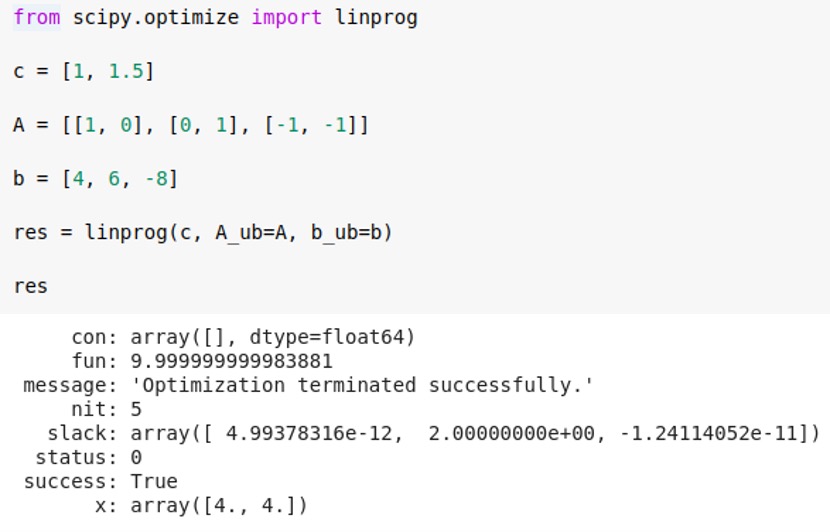Then the objective function will have the form: And constraints function will be: Where vector c = [1, 1.5] is a transportation cost. The matrix A is the coefficients for constraint functions with x11 and x12 for warehouses and plants. And vector b = [4, 6, -8] is the value of raw material on the warehouses and required amount for the plant. As we see from the example, the first warehouse shipped 4 tons of raw materials, and the second warehouse added 4 tons of raw materials. The total cost is 4 + 1.5 * 4 = 10 thousand dollars. This will be the minimum cost of expenses to provide the plant with the right amount of raw materials. Now let's take the following example, which will be a little bit more complicated. There are 3 warehouses and 2 plants. Raw materials are transported from warehouses to plants. The first warehouse has a1 = 4 tons of raw materials. The second warehouse has a2 = 6 tons of raw materials. The third warehouse has a2 = 6 tons of raw materials. The first plant has a need for b1 = 8 tons of raw materials. The second plant has a need for b2 = 8 tons of raw materials. The cost of transportation from all warehouses is the same and equal to 1 thousand dollars. 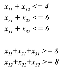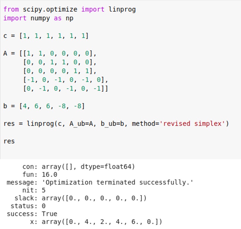Then the objective function will have the form: And constraints function will be: We get this result That is, raw materials from the warehouse 3 and warehouse 1 for 2 and 6 tons, respectively, are brought to the first plant. And raw materials from a warehouse of 2 and warehouse 1 of 4 tons are brought to the second plant. That is, each plant will receive 8 tons of raw materials, as was necessary. Now let’s imagine that the cost of transportation from the first warehouse to the second plant became 2 thousand dollars, for example, in connection with a detour on another road due to the repair of the bridge. Then we set the desired value in the array c = [1, 2, 1, 1, 1, 1]. 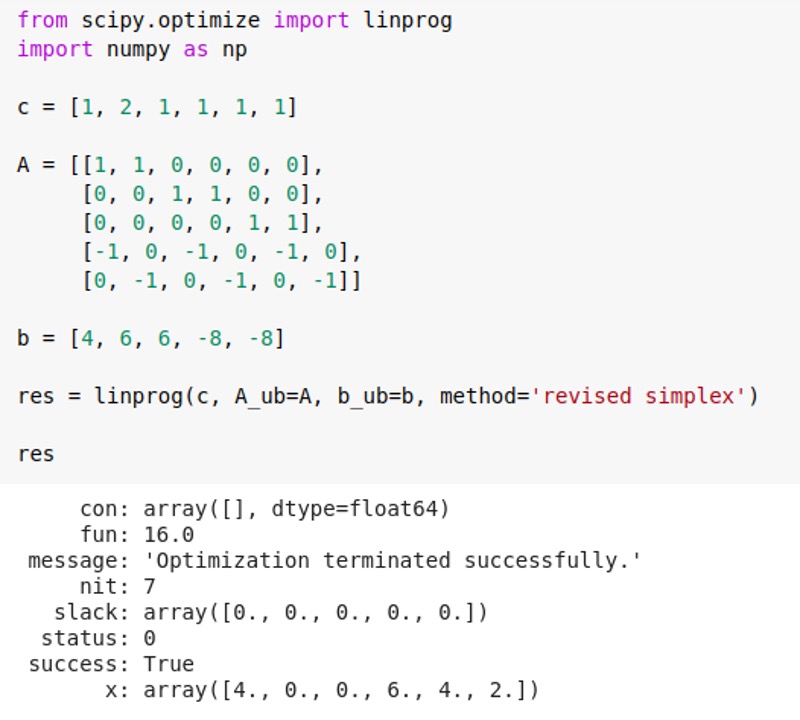And we get the lowest cost of transportation of 16 thousand dollars. Raw materials are brought to the first plant from the first warehouse (4 tons) and from the third warehouse (4 tons).  Raw materials are brought to the second plant from the second warehouse (6 tons) and from the third warehouse (2 tons). In total, both plants will receive 8 tons of raw materials, as required at the lowest possible cost.

Conclusion

In conclusion, we note that linear programming problems are still relevant today. The complexities of optimization in Python are very well developed and have excellent implementation in libraries. They allow you to solve a lot of current problems, for example, in planning project management, economic tasks, creating strategic planning. Our specialists from Svitla Systems are very well versed in solving such problems. This allows us to quickly and efficiently solve the problems encountered by our customers. This example was considered for demonstration, but in fact, this approach allows us to solve problems with millions of components, for example, in a transport problem. With the growth of modern requirements for the implementation of projects in the shortest possible time and with an optimal budget, the task of linear programming can be used in almost all areas. This method is quite simple, but at the same time allows for significant budget savings. Contact Svitla Systems for the necessary advice in the field of datascience and outsourcing of projects in various fields that will be completed reliably and on time.