Math at the Heart of CNN: Part 2

Hello, everyone! My name is Oleksii; I'm a Machine Learning Engineer at Svitla Systems. The previous article, “Using CNNs for Image Processing,” described the motivation behind the development of CNNs, their history, different variants of CNNs, and the current state of the art. However, many aspects remain unclear without a deep understanding of the math behind CNNs. In this article, we will take a closer look at how image filters and convolutional layers work. I hope this will help you better understand how CNNs are used for image processing and improve your skills.

Below you will also find code samples and algorithms for convolutional neural networks. You can rewrite/copy it yourself for your own needs or use the already implemented code in Google Collab for convenience.

Convolutional Operation’s Math

This section will explore convolutional neural networks' mathematical and algorithmic foundations (CNNs). The convolutional operation is the main element distinguishing CNNs from other types of neural networks. This powerful tool allows the network to detect useful features in images regardless of their position, efficiently.

Convolution in CNN applies a filter (or “convolution kernel”) to an image. The filter is a small matrix multiplied by the image's pixels. The filter moves through the image, looking at small areas of the image one by one, which allows us to analyze local features.

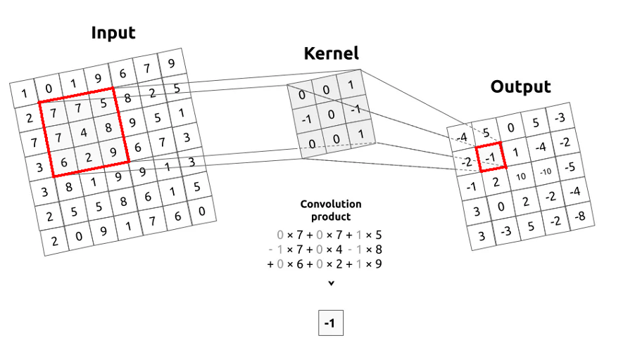
An example of a convolution operation is where a filter is applied to the input image (Input), meaning their values are multiplied and added to form new values for the next image (Output).

Formally, we can define the convolution process as follows:

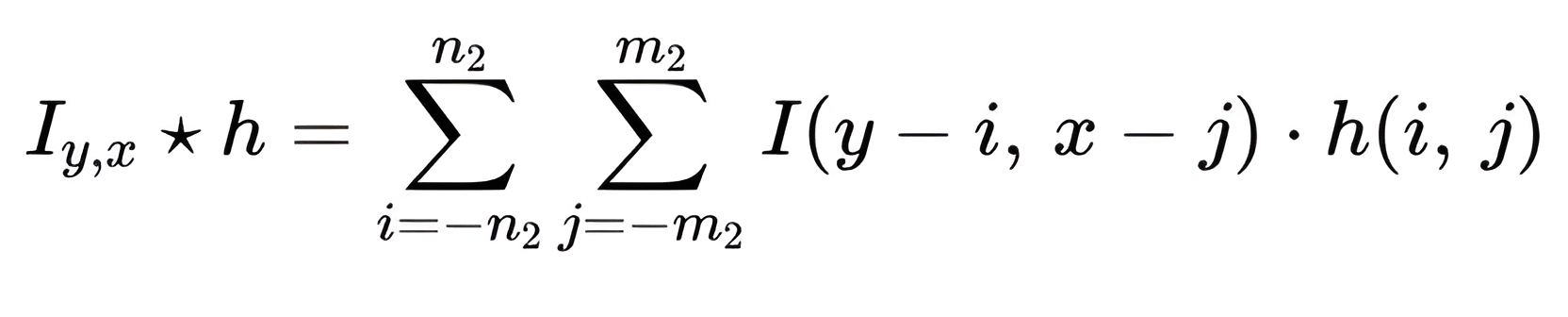
Where:

• n2 is half the height of the filter
• m2 is half the length of the filter
• x is the column position of a certain pixel in the image
• y is the row position of a certain pixel in the image.

By the definition n2 = [n/2], m2 = [m/2] above, n is the height of the filter, and m is the length of the filter h. 

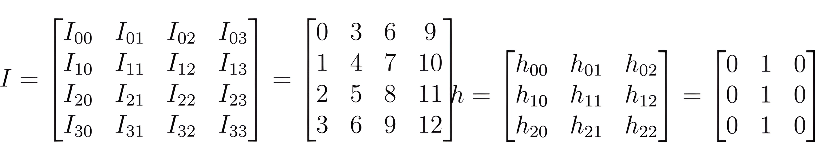
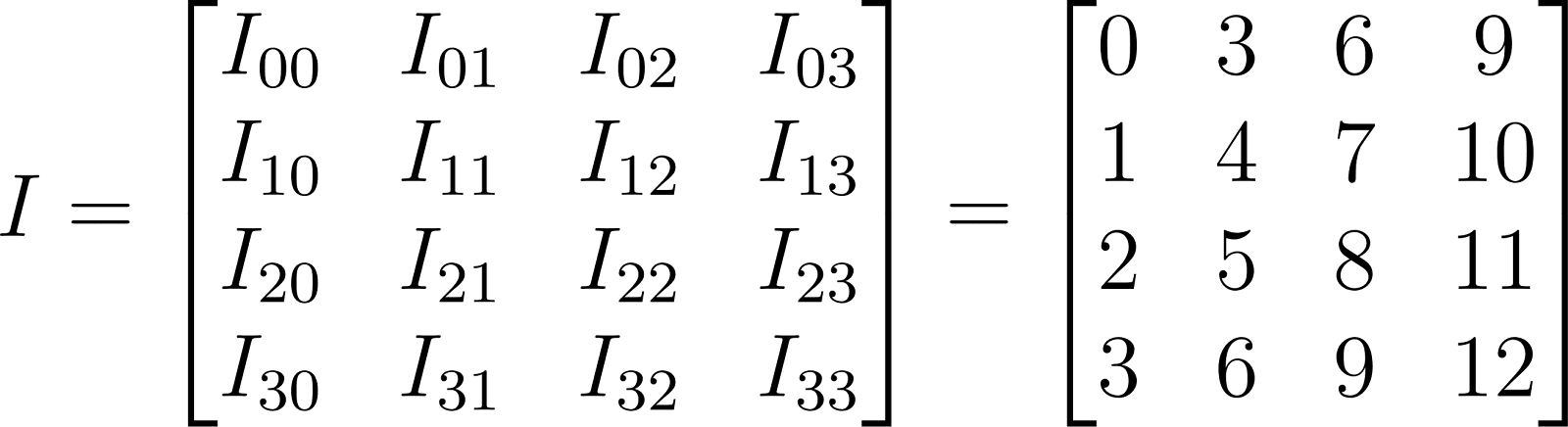
For example, let's take the image I and the filter defined below. We can apply the convolution formula to them.

To apply convolution, you need to define more details about how the filter will move across the input image. The first value you need to define is the increment of how many pixels the values will move in the image. This parameter is called stride.

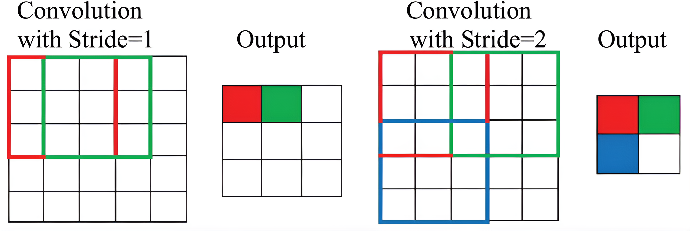
The image on the left shows the filter moving one step, i.e. stride=1. In the image on the left, stride=2, the green area to be processed is two pixels to the right of the red area. Note that the larger the stride value, the smaller the image size.

Source: Analytics Vidhya

The second value is the number of additional rows and columns outside the image, or padding. It is used to determine how much information from the image we want to keep after convolution.

The input image has added rows and columns filled with zeros, i.e. padding=1, and stride=1, so the output image is virtually indistinguishable from the input image.

Source: Analytics Vidhya

As you can see from the examples above, the resulting size and value can vary depending on these two parameters. Therefore, we will assume the values for stride=1 and padding=0 for simplicity. Based on these values, we can calculate the output image size for the matrix we defined earlier. Since its size is 4x4 and the filter we will apply to it is 3x3, the output matrix will have dimensions of 2x2. This value can be calculated using the formula below:

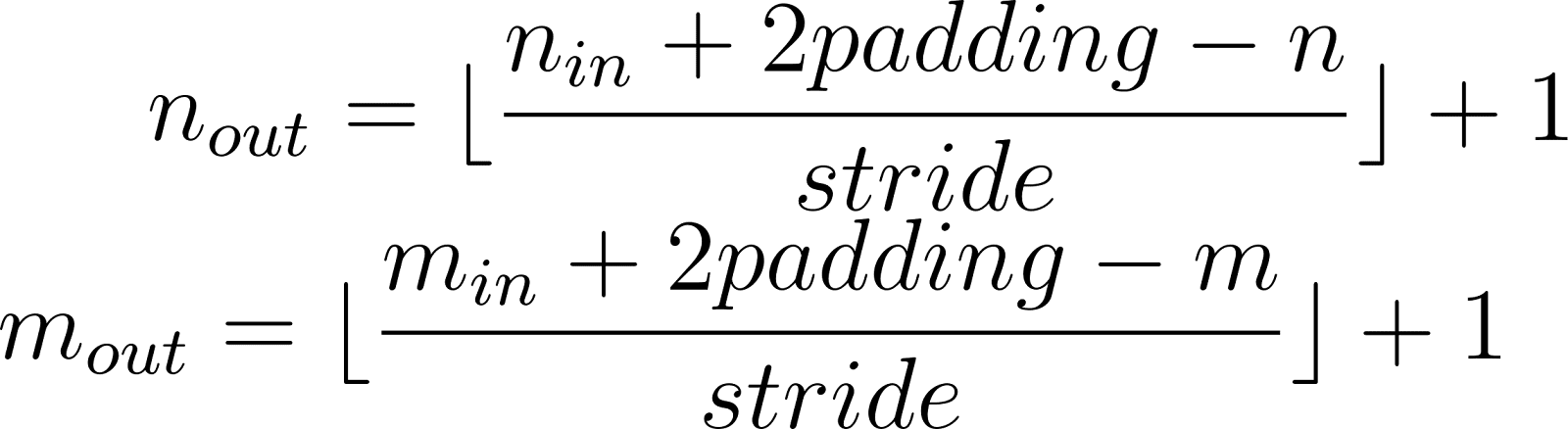
Where n_in, m_in – height and length of the input image,

n_out, m_out – are the height and length of the output image.

So, having all the necessary data, we can start the convolution, which will be performed for the elements I_11, I_12, I21, and I_22 as shown in the figure below:

Find the convolution value for the element I_x=1,y=1 and filter h:

Thus, we can say with certainty that the first element is 12. Accordingly, for the element with coordinates x=2, y=1,  we have the following result:

Thus, the next element has a value of 21. Doing the same operation for the elements I_y=2, x=1; I_y=2, x=2, we can determine that their values are 15 and 24, respectively. As a result of the convolution, we get the following matrix:

Below is a code sample implementing this convolution algorithm in Python:

```python
!wget -O “Lenna_(test_image).png” https://static.wikia.nocookie.net/computervision/images/3/34/Lenna.jpg/revision/latest?cb=20050408081934
# Importing the necessary libraries
import cv2
import numpy as np
import matplotlib.pyplot as plt

# Convolution function
def convolve(img, filter_, k, x, y):
    sum = 0
    # Determine the starting point of the kernel
    k_start = int(-np.floor(k/2))
    # Convolution: multiply the image and filter elements and sum them
    for i in range(k):
        for j in range(k):
            a = img[y+i+k_start][x+j+k_start] * filter_[i][j]
            print(f“i[{y+i+k_start},{x+j+k_start}]*f[{i},{j}]={a} ‘, end=’\t”)
            sum += a
        print(“”)
    # Return the result of convolution for a given point
    return sum

# Kernel size
k = 3
# Filter for convolution
filter_ = [
    [0, 1, 0],
    [0, 1, 0],
    [0, 1, 0],
]
# Input image
img = [
    [0, 3, 6, 9 ],
    [1, 4, 7, 10],
    [2, 5, 8, 11],
    [3, 6, 9, 12]
]
# Determine the height and width of the image
height = len(img)
width = len(img[0])

# Define the boundaries within which the convolution will be performed
row_start = int(np.floor(k/2))
row_end = height-k+2
col_start = int(np.floor(k/2))
col_end = width-k+2

# Create a new image filled with zeros, smaller than the original by the size of the kernel
new_image = np.zeros((height-k+1, width-k+1))
for y in range(row_start, row_end):
    # for x in range(col_start, col_end):
        # Convolve for each point in the area defined by the borders
        new_image[y-row_start][x-col_start] = convolve(img, filter_, k, x, y)
        print(f “process ({x=}, {y=}) image point\n”)

# Print the result of convolution
new_image
```

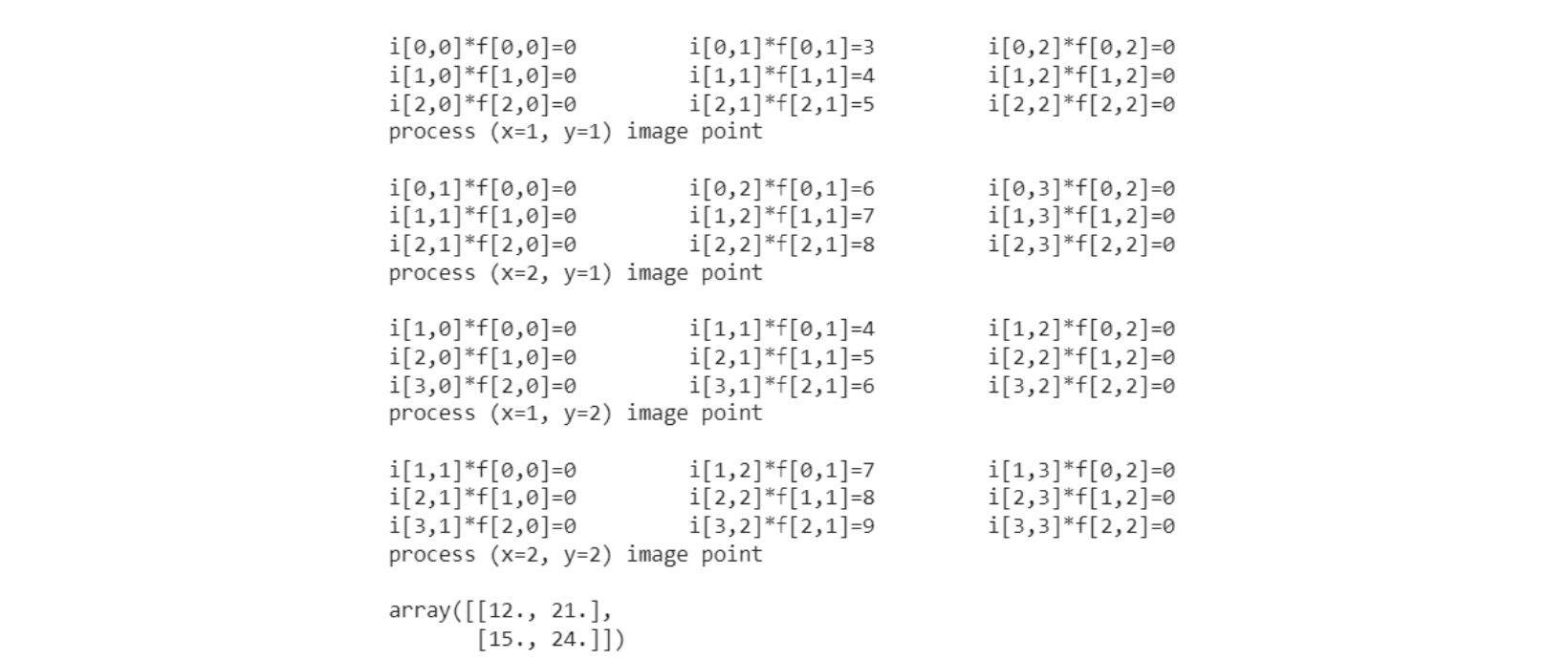
As you can see from the image of the results above, our calculations agree perfectly with the program's algorithm.

Convolution for Black and White Images

Now that we have an idea of what convolution is, how it works, and its implementation, we can apply it to a real image:

```python
# convolution function
def convolve(img, filter_, k, x, y):
    sum = 0
    # Determine the starting point of the kernel
    k_start = int(-np.floor(k/2))
    # Convolution: multiply the image and filter elements and sum them
    for i in range(k):
        for j in range(k):
            sum += img[y+i+k_start][x+j+k_start] * filter_[i][j]
    # Return the result of convolution for a given point
    return sum

# Convolution function for the entire image
def convolve_image(img, filter_):
    # Determine the size of the kernel
    k = filter_.shape[0].
    # Define the boundaries within which convolution will be performed
    row_start = int(np.floor(k/2))
    row_end = height-k+2
    col_start = int(np.floor(k/2))
    col_end = width-k+2
    # Create a new image filled with zeros, smaller than the original by the size of the kernel
    new_image = np.zeros((height-k+1, width-k+1))
    for y in range(row_start, row_end):
        # for x in range(col_start, col_end):
            # Convolve for each point in the area defined by the borders
            new_image[y-row_start][x-col_start] = convolve(img, filter_, k, x, y)
    return new_image

# Load the image
img = cv2.imread('Lenna_(test_image).png', 0)
height, width = img.shape

# Create a figure with 2 graphs
fig, axs = plt.subplots(ncols=2, nrows=1, figsize=(14, 6))

# Define the size and type of filter

“””
For k = 3, the filter will look like this:
[[0, 1, 0],
 [0, 1, 0],
 [0, 1, 0]],
“””
k = 15
filter_ = np.zeros((k, k), dtype=int)
filter_[:, k // 2] = 1

# Convolve the image
new_image = convolve_image(img, filter_)

# Display the original and convolved image
axs[0].imshow(img, cmap='gray')
axs[1].imshow(new_image, cmap='gray')

# Display the graphs
plt.show()
```

In the example above, I chose a size for the filter of 15 to reflect better the difference between the original image and the one that has been convolved. That's why we have the result below:

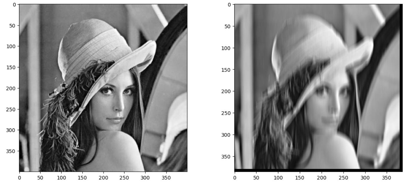
Since the output image is smaller than the input image, we can see black bars (bottom and right) in the image on the right, which are zeros.

This code performs image convolution using a vertical 2D filter (Sobel filter). The Sobel filter is used to detect edges in an image.

This filter mainly detects vertical edges because it has non-zero values in the middle column. Thus, after applying this filter to the image, the vertical edges will be more highlighted.

This code's result is two images: the original image and the image after convolution. After convolution, the image will reflect the detected edges in the original image.

In the example below, I've shown you other ways to apply different versions of this filter to give you a better impression of how this algorithm works.

```python
def convolve(img, filter_, k, x, y):
    """
    Optimized image convolution function
    “””
    # Determine the starting point of the kernel
    k_start = int(-np.floor(k/2))
    # Cut a fragment of the image the size of the kernel
    img_slice = img[y+k_start:y+k_start+k, x+k_start:x+k_start+k]
    # Multiply the image slice and the kernel and sum the result
    return np.sum(np.multiply(img_slice, filter_))

# We are quantifying the image
img = cv2.imread('Lenna_(test_image).png', 0)
img.shape

# Kernel size
k = 25
# Filter 1
"""
[[0, 1, 0],
 [0, 1, 0],
 [0, 1, 0]],
"""
filter1 = np.zeros((k, k), dtype=int)
filter1[:, k//2] = 1

# Filter 2
"""
[[0, 0, 0],
 [1, 1, 1],
 [0, 0, 0]],
"""
filter2 = np.zeros((k, k), dtype=int)
filter2[k//2, :] = 1

# Filter 3
"""
[[1, 0, 0],
 [0, 1, 0],
 [0, 0, 1]],
"""
filter3 = np.zeros((k, k), dtype=int)
np.fill_diagonal(filter3, 1)

# Filter 4
"""
[[0, 0, 1],
 [0, 1, 0],
 [1, 0, 0]],
"""
filter4 = np.zeros((k, k), dtype=int)
np.fill_diagonal(np.fliplr(filter4), 1)

# Filter 5
“””
[[1, 1, 1],
 [1, 0, 1],
 [1, 1, 1]],
“””
filter5 = np.ones((k, k))
if k > 2:
    filter5[1:-1, 1:-1] = 0

# List with all filters
filters = [filter1, filter2, filter3, filter4, filter5]

# Filter names
filter_names = ['|', '-', '\\', '/', '□' ]

# Create a figure to display the graphs
fig, axs = plt.subplots(ncols=3, nrows=2, figsize=(14, 9))

# Display the original image
axs[0, 0].imshow(img, cmap='gray')
axs[0, 0].set_title('Original Image')

# Apply each filter to the image and display the result
for i, filter_ in enumerate(filters):
    new_image = convolve_image(img, filter_)
    axs[(i+1)//3, (i+1)%3].imshow(new_image, cmap='gray')
    axs[(i+1)//3, (i+1)%3].set_title(f'Filter {i+1}, {filter_names[i]}')

# Show the graphs
plt.show()
```

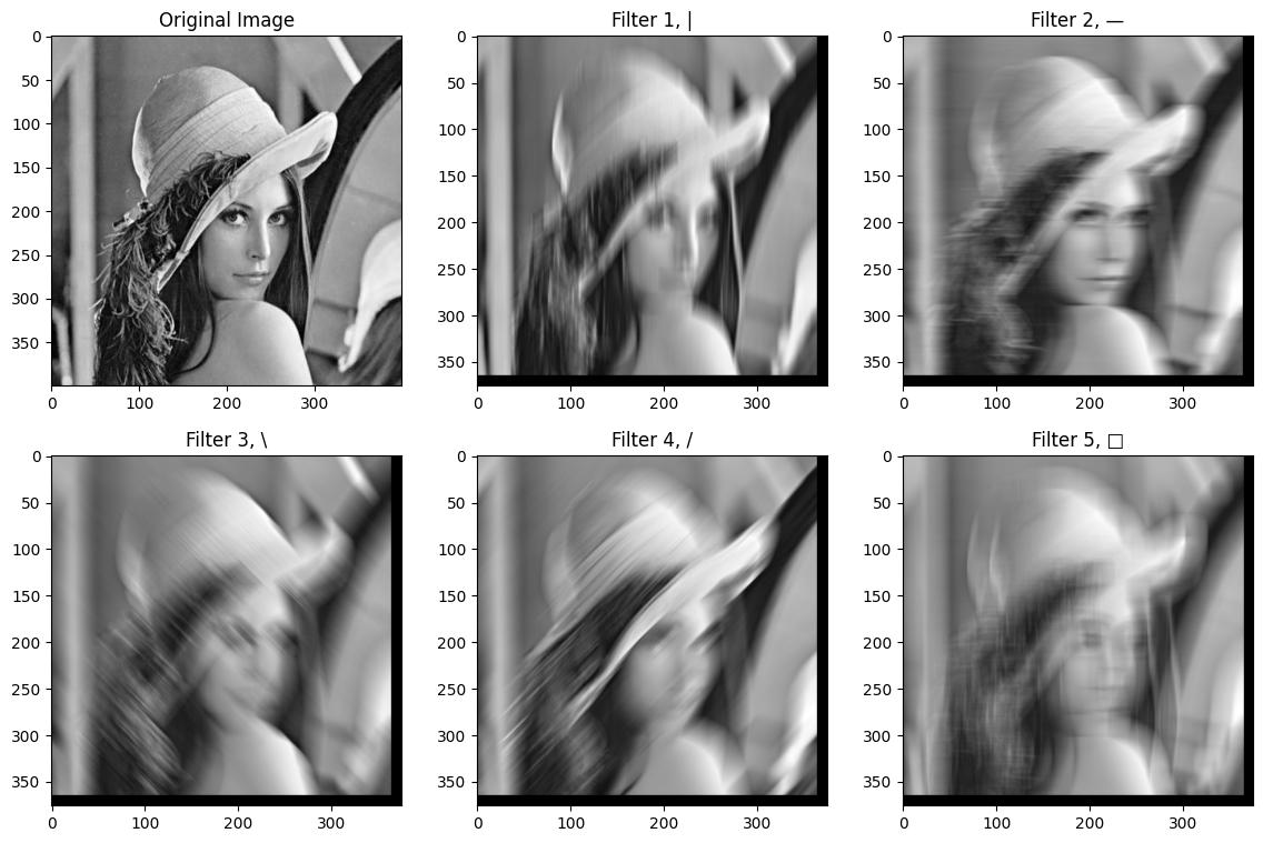
An example of applying vertical, horizontal, and slanted lines to an image.

This code applies various filters to the input image and visualizes the results.

• Filter 1 (|): This filter highlights vertical lines in the image. The result is an image where vertical lines are more prominent.
• Filter 2 (-): This filter emphasizes horizontal lines in the image. The result is an image where horizontal lines are more prominent.
• Filter 3 (\): This filter highlights diagonal lines running from the top left to the bottom right corner. The result is an image where these diagonal lines are more prominent.
• Filter 4 (/): This filter highlights the diagonal lines that run from the top right corner to the bottom left corner. The result is an image where these diagonal lines are more prominent.
• Filter 5 (□): This filter emphasizes the edges of objects in the image. The result is an image where the edges of objects are more prominent.

As you can see, different filters can get their features, and this concept is the basis for building modern convolutional neural networks.

Pulling for Black and White Images

We have considered the mathematical and algorithmic aspects of the first part of convolutional networks, namely the convolution operation. The next task is to formulate a mathematical and algorithmic description of the second part of convolutional networks, i.e., the pooling operation. Consider, for example, the maximization operation, or max-pooling, which can be formulated as follows:

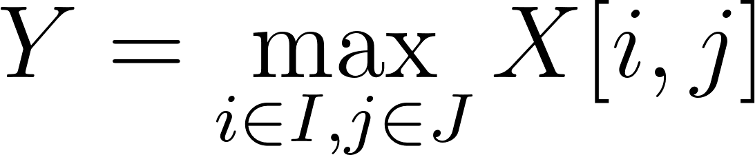
Where:

The formula takes the maximum of all elements of the pooling window in X and assigns this value to the corresponding element in Y.

So, we look at each window of the input image of size I X J, starting at position (i,j), and select the maximum value from that window.

Now let's look at an example of how this works. For example, we have a matrix that looks like this:

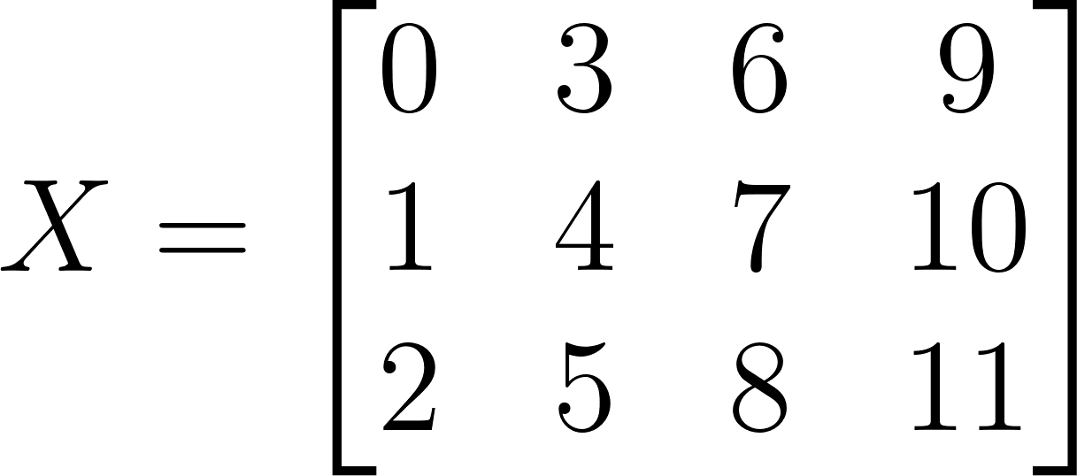
Now we can apply the pooling operation to it. For example, let's use a pooling window of 2 and a stride, a window step with a value of one. Then the areas for which the max-pooling operation will be used will look like this:

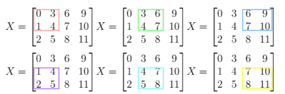
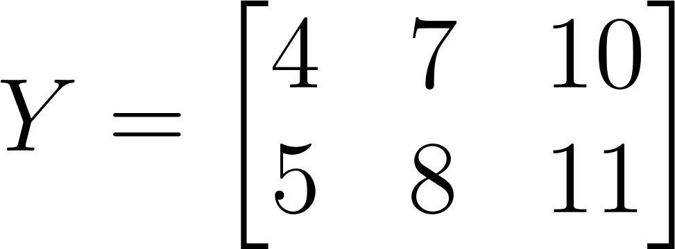
As you can see in the image above, the processing results in a 2×3 matrix. Thus, the matrix will look like this:

By implementing this logic in the algorithm after using convolution, the code below demonstrates a clearer highlighting of the image's strong features.

```python
def max_pooling(img, k, x, y):
    """
Function for performing max-pulling on the input image img
    with kernel size k and output values x, y
    “””
    # Determine the starting point for the kernel
    k_start = int(-np.floor(k/2))
    # Get an image from the range y+k_start:y+k_start+k, x+k_start:x+k_start+k
    img_slice = img[y+k_start:y+k_start+k, x+k_start:x+k_start+k]
    # Return the maximum value of this image
    return np.max(img_slice)

def max_pooling_image(img, k, stride=1):
    """
   height, width = img.shape
    # Define start and end points for rows and columns
    row_start = int(np.floor(k/2))
    row_end = height-k+2

    col_start = int(np.floor(k/2))
    col_end = width-k+2

    # Initialize the image after pooling
    pooled_image = np.zeros()
        np.floor((height-k)/stride).astype(“int”) + 1,
        np.floor((width-k)/stride).astype(“int”) + 1
    ))
    # Iterate through each pixel of the image
    for i, y in enumerate(range(row_start, row_end, stride)):
        for j, x in enumerate(range(col_start, col_end, stride)):
            # Perform max-pooling for the current window
            pooled_image[i][j] = max_pooling(img, k, x, y)
    # Return the image after pooling
    return pooled_image

# Input image
img = np.array([
    [0, 3, 6, 9 ],
    [1, 4, 7, 10],
    [2, 5, 8, 11]
])
height, width = img.shape # Get the size of the input image

# Kernel size
k=2
# Performing maximum image pooling
pooled_image = max_pooling_image(img, k)
pooled_image # Display the image after pooling
```

As a result of executing this code, we will get the result shown below.

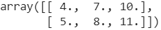
Now, we can see the result of combining the above functions, i.e., the convolution and pooling operations for processing black-and-white images.

Python.
# Load the image in black and white format
img = cv2.imread('Lenna_(test_image).png', 0)
# Get the dimensions of the loaded image
height, width = img.shape

# Create a shape object to display images
fig, axs = plt.subplots(ncols=3, nrows=1, figsize=(14, 4))

# Set the kernel size for convolution
k_convolve = 15
# Create a filter for convolution
filter_ = np.zeros((k_convolve, k_convolve), dtype=int)
filter_[:, k // 2] = 1
# Convolve the image with the created filter
new_image = convolve_image(img, filter_)

# Set the kernel size for pooling
k_pooling = 10
# Perform a pooling operation on the image after convolution
pooled_image = max_pooling_image(new_image, k_pooling, k_pooling)

# Display the original image
axs[0].imshow(img, cmap='gray')
# Display the image after convolution
axs[1].imshow(new_image, cmap='gray')
# Displaying the image after pulldown
axs[2].imshow(pooled_image, cmap='gray')
# Display all images
plt.show()
```

By executing this code, we get the following result:

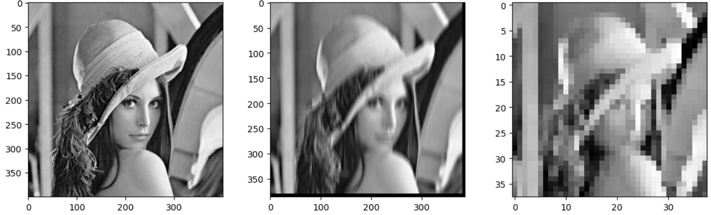
The illustration shows that the first image is the original, the second is the one processed using convolution, and the third is after applying the max-pooling function.

As you can see from the last image, which has undergone max-pooling, the image dimension has been significantly reduced because the kernel and padding parameters for the pooling operation were set to 10. Thus, we extracted the features calculated by the convolutional filter and composed a less detailed image. However, if we had several similar convolution filters that received vertical and horizontal features, we would have saved more information for further processing.

Compression and Pulldown for Color Images

So far, all the examples I've shown you have been for black-and-white images.  Now we'll look at how these operations work with RGB color images. We used the convolution operation for black-and-white images and performed it on specific positions in the image. We can describe the convolution for the entire single-channel image as I * h. The convolution for a multichannel image will look like this:

Where:

• I_in – input image,
• I_out is the output image,
• C_in is a number of channels in the input image,
• c is image channel index, in the case of RGB, it will be a red, green, or blue channel.

In other words, according to the formula above, passing a multichannel image to the input results in a single-channel image. In the case of a color RGB image, the output will be a black-and-white image. This is exactly what we can see as a result of implementing this formula.

```python
def convolve_RGB_image(img, filter_):
    height, width, channels = img.shape
    # Initialize the source image
    new_image = np.zeros((height, width), dtype=np.float64)

    # Apply convolution
    for y in range(k//2, height - k//2):
        for x in range(k//2, width - k//2):
            for c in range(channels):
                new_image[y, x] += convolve(img[:,:,c], filter_, k, x, y)

    # Normalize the image to 8-bit format
    new_image = (new_image / np.max(new_image) * 255).astype('uint8')
    return new_image

# Load the image
img_original = cv2.imread('Lenna_(test_image).png')
img_original_RGB = cv2.cvtColor(img_original, cv2.COLOR_BGR2RGB)

# Initialize the filter
k = 25
filter_ = np.zeros((k, k), dtype=int)
filter_[:, k // 2] = 1

new_image = convolve_RGB_image(img_original_RGB, filter_)

# Show the original and collapsed image
fig, axs = plt.subplots(ncols=2, nrows=1, figsize=(14, 6))

axs[0].imshow(img_original_RGB)
axs[0].set_title('Original image')

axs[1].imshow(new_image, cmap=“gray”)
axs[1].set_title('Image after convolution')

plt.show()
```

In the example above, the convolve_RGB_image function contains image normalization so that the resulting single-channel image can be displayed in the black-and-white spectrum, and the following result can be obtained.

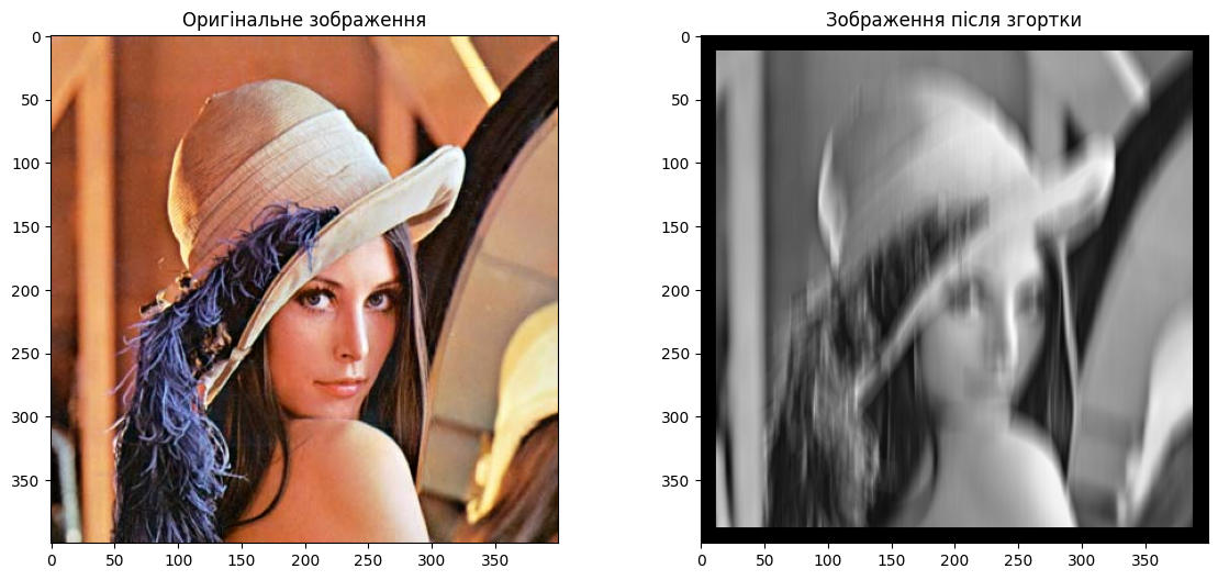
Code execution occurs after a convolution operation converts a color image to black and white.

Now we can combine the convolution algorithm with the pooling algorithm.

Where:

• I_0 is the input image,
• I_1 is the image after convolution on all input channels,
• I_2 is image after max-pulling.

```python
# Load the image
img_original = cv2.imread('Lenna_(test_image).png')
img_original_RGB = cv2.cvtColor(img_original, cv2.COLOR_BGR2RGB)


# Initialize the filter
k = 25
filter_ = np.zeros((k, k), dtype=int)
filter_[:, k // 2] = 1
# Initialize the output image
convolved_image = convolve_RGB_image(img_original_RGB, filter_)


# Apply max_pooling
pool_size = 10
pooled_image = max_pooling_image(convolved_image, pool_size, pool_size)


# Show the original, collapsed, and the image after max_pooling
fig, axs = plt.subplots(ncols=3, nrows=1, figsize=(21, 7))

axs[0].imshow(img_original_RGB)
axs[0].set_title('Original image')

axs[1].imshow(convolved_image, cmap=“gray”)
axs[1].set_title('Image after convolution')

axs[2].imshow(pooled_image, cmap=“gray”)
axs[2].set_title('Image after max_pooling')

plt.show()
```

Combining the color convolution and max-pooling algorithms gives us a complete picture of how convolutional layers work and how they allow us to extract certain features from images.

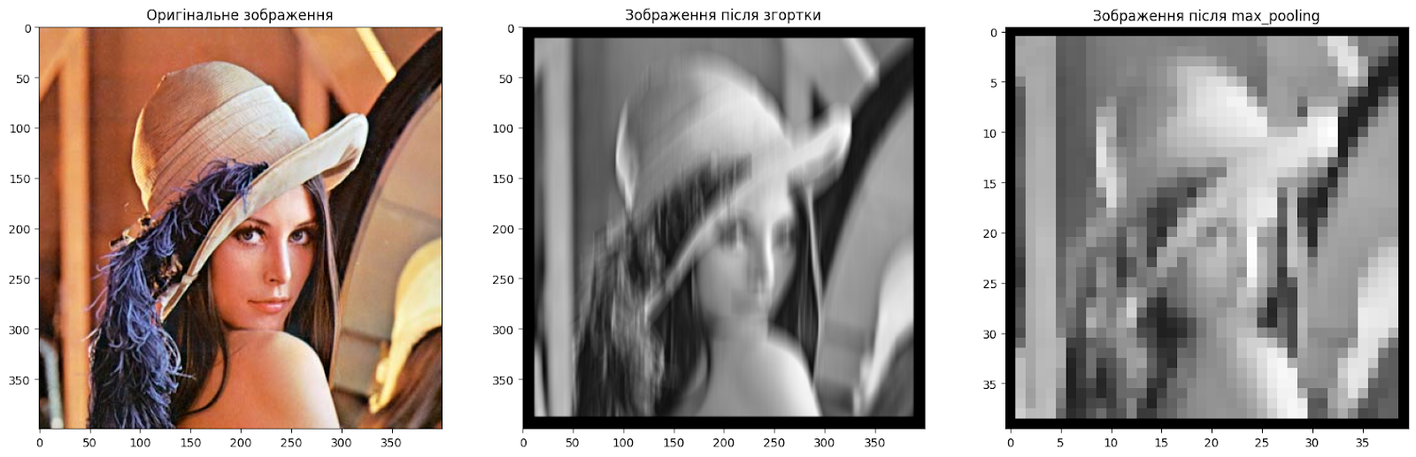
We can obtain various image characteristics by having many filters with different values that process color images.

Neural Networks Based on Convolution and Pooling

So far, we have seen the convolutional operation for color images and the max-pulling operation. With all this information, we can now easily derive the concept of convolutional neural networks. First, we can use matrices with randomly generated values w or weights instead of a predefined hfilter.  The more such filters there are, the more different features we can extract from the images. By determining the number Cout of filters to process, we can get the same number of single-channel images at the output or one image with Cout channels.

In addition, some features may stand out more clearly than others, creating noise that will hide features that may be important for this particular task. That's why we add a vector bias (Cout), which allows you to compensate for the convolutional layer's predisposition to some features and bypass others (for details, see the documentation of the PyTorch library convolutional layers).

Since these operations are linear, no matter how deep any convolutional network is, it could be reduced to a single layer since the composition of linear functions is linear. That is why the concept of the activation function Activation (•) is introduced. Activation functions introduce nonlinearity into the model, allowing the neural network to learn and model more complex functions and patterns in the data. They determine the output of a node (neuron) in the network. The application of an activation function involves transforming the output of a neuron so that it can be used as an input to the next layer of neurons.

In convolutional neural networks, the ReLU (Rectified Linear Unit) activation function is often used because it helps the model converge faster during training and effectively handles the problem of gradient washout that can occur with other activation functions, such as sigmoid or hyperbolic tangent. Once we have the output from this function, we can use pooling.

This is the complete formula for describing a single layer of a convolutional network. By overlaying, layer by layer, convolutional neural networks can extract more and more complex features from an image. This is how deep convolutional neural networks are built.

The first successful neural network used to solve real-world problems, namely to recognize handwritten postal codes, was the LeNet network, named after the implementer Jan LeCun, developed in 1989. You can see an example of its work in the video below:

Next is the architecture of this neural network, which is implemented using the PyTorch library:

```python
#Означення згорткової нейронної мережі
class LeNet5(nn.Module):
    def __init__(self, num_classes):
        super(ConvNeuralNet, self).__init__()
        self.layer1 = nn.Sequential(
            nn.Conv2d(1, 6, kernel_size=5, stride=1, padding=0),
            nn.BatchNorm2d(6),
            nn.ReLU(),
            nn.MaxPool2d(kernel_size=2, stride=2))
        self.layer2 = nn.Sequential(
            nn.Conv2d(6, 16, kernel_size=5, stride=1, padding=0),
            nn.BatchNorm2d(16),
            nn.ReLU(),
            nn.MaxPool2d(kernel_size=2, stride=2))
        self.fc = nn.Linear(400, 120)
        self.relu = nn.ReLU()
        self.fc1 = nn.Linear(120, 84)
        self.relu1 = nn.ReLU()
        self.fc2 = nn.Linear(84, num_classes)
        
    def forward(self, x):
        out = self.layer1(x)
        out = self.layer2(out)
        out = out.reshape(out.size(0), -1)
        out = self.fc(out)
        out = self.relu(out)
        out = self.fc1(out)
        out = self.relu1(out)
        out = self.fc2(out)
        return out
```

As you can see, the architecture consists of two layers of convolutional neural networks and three layers of conventional artificial neurons. Each convolutional layer has the functions we mentioned earlier and increases the number of channels at the output of each layer. The first layer converts a black-and-white image into a six-channel image, and the second layer converts a six-channel image into a 16-channel image.

But the real novelty of this neural network was that the filters implemented were weights that changed during training. For them, a backpropagation algorithm was implemented (for those interested in the details, see the video here).

This was the basis for the further development and revolution of the entire field of computer vision, which broke out in 2012 with the release of another well-known neural network, AlexNet.

Conclusion.

In this article, we have reviewed the main mathematical principles behind convolutional neural networks. We have analyzed the convolutional operation in detail, found out how it is applied to black and white and color images, and also considered pooling. The main goal of this article is to help readers better understand how convolutional neural networks work, not to demonstrate their optimal implementation in modern libraries.

We didn't have time to consider the details of the backpropagation algorithm, filter initialization, kernel size, etc., which are also important elements of neural network training. Nevertheless, I hope this article has given you a sense of the basic principles of CNN. So, you gained new and useful information that will help you better understand and use, perhaps even, your convolutional neural networks.