We are witnessing an intensive use of numerical methods across different modern fields of science and technology.

Why? A wide variety of applied problems can be solved using calculation methods that are based on mathematical principles using digital values as opposed to analytical and symbolic methods.

For example, when solving engineering problems, it is relatively common to use the calculation of the derivative of a function.

In data science, it’s no different. Oftentimes, input values of functions are specified in the form of an argument-value pair, which in large data arrays, can be significantly data-intensive to process. Fortunately, many problems are much easier to solve if you use the derivative of a function, helping across different fields like economics, image processing, marketing analysis, etc.

Computation of derivatives is often used in data analysis. For example, when finding the optimum of the values of functions. The calculation of the derivative is also used for gradient methods when training neural networks.

In this post, we examine how you can calculate the value of the derivative using numerical methods in Python.

Table of contents:

1. Numerical Differentiation Principle.
2. Python Methods for Numerical Differentiation.
3. Error Estimate with an Analytical Form of Differential.
4. Conclusion.

Numerical Differentiation Principle

Numerical differentiation is based on the approximation of the function from which the derivative is taken by an interpolation polynomial. All basic formulas for numerical differentiation can be obtained using Newton's first interpolation polynomial.

The general formula to calculate the derivative is:

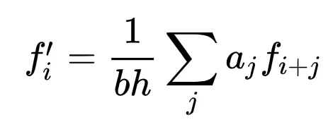
Here, the coefficients aj and b depend on the n degree of the used interpolation polynomial, that is, on the required accuracy. Coefficients up to the 5th order can be presented in the form of a table:

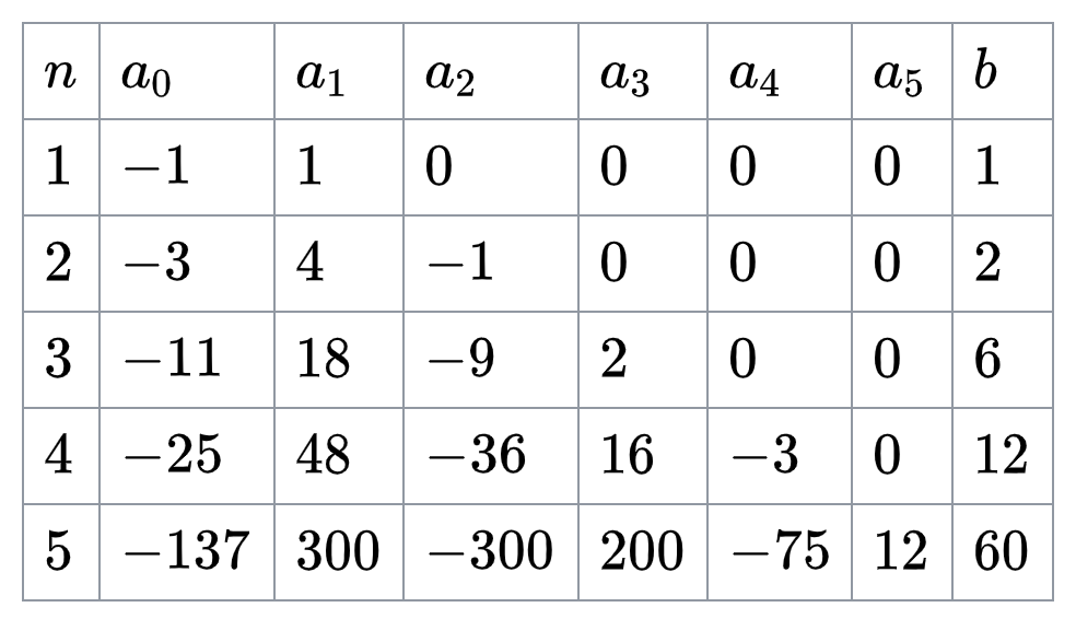
You can easily get a formula for the numerical differentiation of a function at a point by substituting the required values of the coefficients.

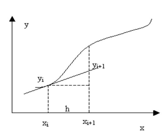
For example, Euler's method which the simplest numerical method for solving systems of ordinary differential equations, will look like this

Euler's method can be graphically represented as follows:

Python Methods for Numerical Differentiation

For instance, let’s take the function y = f (x), y = x2. Then, let’s set the function value in the form of pairs x, y with a step of 0.01 for the range of x from 0 to 4.

We’re going to use the scipy derivative to calculate the first derivative of the function. Please don’t write your own code to calculate the derivative of a function until you know why you need it. Scipy provides fast implementations of numerical methods and it is pre-compiled and tested across many use cases.

import numpy
import matplotlib.pyplot as plt
 
def f(x):
 return x*x
 
x = numpy.arange(0,4,0.01)
y = f(x)
 
plt.figure(figsize=(10,5))
plt.plot(x, y, 'b')
plt.grid(axis = 'both')
plt.show()
Code language: JavaScript (javascript)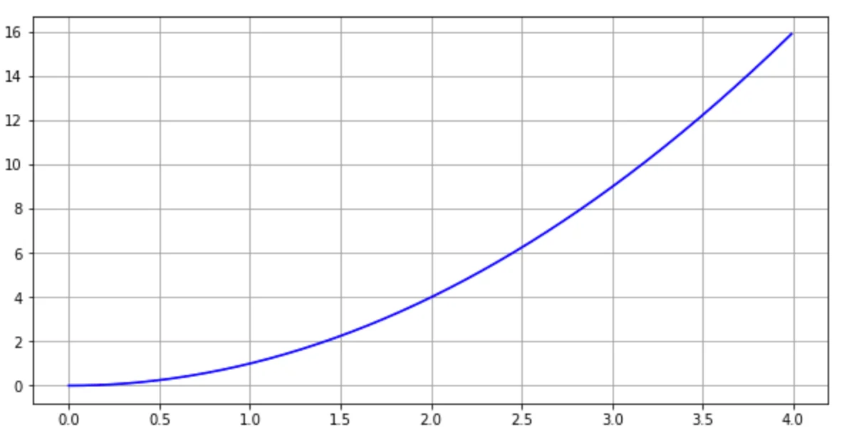

Now, let's take a function from the scipy.misc library and calculate the value of the derivative at the point x = 1. Let’s set the derivation step of the method to 0.001.

To get more information about scipy.misc.derivative, please refer to this manual. It allows you to calculate the first order derivative, second order derivative, and so on. It accepts functions as input and this function can be represented as a Python function. It is also possible to provide the “spacing” dx parameter, which will give you the possibility to set the step of derivative intervals.

# https://docs.scipy.org/doc/scipy-0.18.0/reference/generated/scipy.misc.derivative.html
#
from scipy.misc import derivative
 
d = derivative(f, 1.0, dx=1e-3)
 
print (d)

1.9999999999998352
Code language: PHP (php)

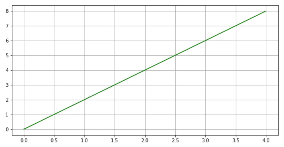
Also, you can use the library numpy to calculate all derivative values  in range x = 0..4 with step 0.01 as we set in the input function. Then, you can use the np.gradient method. 

import numpy as np
 
dy = np.gradient(y)
dx = np.gradient(x)
 
d = dy/dx
d
 
array([0.01, 0.02, 0.04, 0.06, 0.08, 0.1 , 0.12, 0.14, 0.16, 0.18, 0.2 ,
       0.22, 0.24, 0.26, 0.28, 0.3 , 0.32, 0.34, 0.36, 0.38, 0.4 , 0.42,
       0.44, 0.46, 0.48, 0.5 , 0.52, 0.54, 0.56, 0.58, 0.6 , 0.62, 0.64,
     ...
       7.26, 7.28, 7.3 , 7.32, 7.34, 7.36, 7.38, 7.4 , 7.42, 7.44, 7.46,
       7.48, 7.5 , 7.52, 7.54, 7.56, 7.58, 7.6 , 7.62, 7.64, 7.66, 7.68,
       7.7 , 7.72, 7.74, 7.76, 7.78, 7.8 , 7.82, 7.84, 7.86, 7.88, 7.9 ,
       7.92, 7.94, 7.96, 7.97])
Code language: JavaScript (javascript)

You can also use this option to get a slightly more accurate result than the previous option.

import numpy as np
 
np.gradient(y, x)

array([0.01, 0.02, 0.04, 0.06, 0.08, 0.1 , 0.12, 0.14, 0.16, 0.18, 0.2 ,
       0.22, 0.24, 0.26, 0.28, 0.3 , 0.32, 0.34, 0.36, 0.38, 0.4 , 0.42,
       0.44, 0.46, 0.48, 0.5 , 0.52, 0.54, 0.56, 0.58, 0.6 , 0.62, 0.64,
      ...
       7.26, 7.28, 7.3 , 7.32, 7.34, 7.36, 7.38, 7.4 , 7.42, 7.44, 7.46,
       7.48, 7.5 , 7.52, 7.54, 7.56, 7.58, 7.6 , 7.62, 7.64, 7.66, 7.68,
       7.7 , 7.72, 7.74, 7.76, 7.78, 7.8 , 7.82, 7.84, 7.86, 7.88, 7.9 ,
       7.92, 7.94, 7.96, 7.98, 7.99])
Code language: JavaScript (javascript)

If you look at the graph of the derivative function, you get the following form.

Error Estimate with an Analytical Form of Differential

An error estimate to calculate the derivative’s numerical value can be done by calculating the formula for the derivative in an analytical way and substituting the value at a desired point.

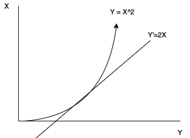
For example, for the function we are considering in this example, you can analytically calculate the formula as follows:

y = x2

y ‘ = 2 x

Then, at point x = 4, you will obtain the value of the derivative 8. Numerical methods from previous yielded 7.97 and 7.99 results, which is due to the approximation of the derivative.

The calculated value using the above methods may differ by approximately 0.01. What’s the reason for this discrepancy?

First, you need to choose the correct sampling value for the function. The smaller the step, the more accurate the calculated value will be.

Second, you must choose the order of the integration function similar to the degree of the polynomial of the function being differentiated.

You also need to consider the region of the absolute stability for the given methods of numerical differentiation. For instance, backward and forward Euler methods can show different stability regions, i.e., it is necessary to have a small differentiation step. Please find more information here.

In addition to scipy differentiate, you can also use analytical differentiation in Python. The SymPy package allows you to perform calculations of an analytical form of a derivative. In some cases, you need to have an analytical formula for the derivative of the function to get more precise results. Symbolic forms of calculation could be slow on some functions, but in the research process, there are cases where analytical forms give advantage compared to numerical methods.

Conclusion

The rapidly developing field of data science and machine learning requires field specialists who master algorithms and computational methods.

Python is a great ally when solving these types of problems thanks to its developed network of libraries and frameworks.

Knowledge of basic numerical methods is essential in this process. Svitla Systems specialists have profound knowledge in this area and possess extensive practical experience in problem-solving in the field of data science and machine learning.

Request expert help and project development at Svitla Systems, where you will always receive qualified services and quality products.