Interpreting Machine Learning Models Using LIME and SHAP

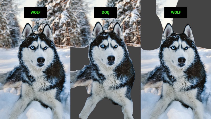
You are seeing three images of a Husky dog lying on the snow. The image on the left side is incorrectly labeled as a wolf; the image in the middle has the snow cropped out but it’s correctly labeled as a dog; the image on the right has trees cropped out and the dog is once again mislabeled as a wolf instead of a dog. 

Table of contents:

1. Why interpreting models is important.
2. The trade-off between prediction accuracy and model interpretability.
3. What is LIME?
4. LIME in Python.
5. What is SHAP?
6. SHAP in Python (linear regression example).
7. Key takeaways.
8. Words of caution.

Why interpreting models is important

When someone acts autonomously, it’s important to understand how and why they make decisions. How does a judge reach a decision when determining if someone’s guilty or not? How do doctors decide on a specific treatment? Why does a screenwriter decide to kill a main character at the end of a season? 

In the near future, we can expect Artificial Intelligence (AI) models to take over decision-making tasks such as lawsuits, non-urgent patient care, or screenwriting. But before we get there, we need to thoroughly understand how and why a decision was reached. Unlike humans, machine learning models cannot be interviewed to understand the motives behind their decision-making processes, and even if we could interrogate them, we would be unable to hold them accountable for the decisions they made in the past. For these reasons, it is crucial to leverage methods that explain model predictions.

Let’s take banking for instance. Risk analysis uses AI models to assign credit scores to applicants and thus, decide whether or not to lend them money—applications with low scores are rejected and applications with high scores are accepted. These scores are generated by processing applicant data such as age, reported income, existing credits on record, and more. 

Imagine if an applicant with a high score requests a very large sum of money. Bankers are known for playing it safe, and applications for large sums of money are likely to be thoroughly reviewed even if scores are high. Particularly, analysts are interested in knowing if the predicted scores from the AI model are a true reflection of the client’s ability and willingness to pay. They’re also interested in knowing if a vulnerability in the model or distortions in the data cause it to predict such a high score for the applicant. Within this context, understanding and explaining the decision-making process behind the AI model matters because there’s a lot of money on the line. Lending money to people who are unlikely to pay it back can have a serious and negative effect on financial institutions and the humans working for them. 

AI models are used to predict outcomes in our everyday lives. In marketing, analysts employ user search history to recommend products to users that they are likely to buy; in the field of medicine, organ scans help predict the likelihood of a specific disease; in gaming, player attributes help match gamers with players of similar skill levels.

Case in Point: Machine Learning Became a Competitive Advantage for Logitech's Video Conferencing Software

Regardless of the industry, analysts are interested in explaining how predictions are made by AI models to determine whether they can be trusted. The methods introduced in this article will help you disentangle the logic behind any model, whether it uses language, images, or tabular data to make predictions. Additionally, you will learn how to apply these methods using Python. The code presented in this article can also be found in this GitHub repository.

The trade-off between prediction accuracy and model interpretability

Generally speaking, complex models tend to make more accurate predictions than simpler models. However, understanding the logic behind a model’s predictions becomes increasingly difficult as we increase its complexity.

It’s easy to understand how a marginal increase in one of the input variables affects the predictions made by a linear regression model(1). Unfortunately, there are times when the relationship between the features and an outcome cannot be accurately predicted by a linear model, so we have to move on to more complex algorithms. Although the predictions made by, say, an ensemble of gradient boosted trees(2) could accurately model a nonlinear relationship, understanding why a prediction came out as it did is not as simple as before.

The accuracy gained by using an ensemble method is offset by the loss in interpretability of the new model. This is the essence of the infamous accuracy-interpretability trade-off.

What is LIME?

Not long ago, we used to think this trade-off was inevitable. Fortunately, researchers have proposed a few methods that can help us understand the logic behind the predictions made by any model, no matter how complex.

Local Interpretable Model-agnostic Explanations, also known as LIME, was proposed by Marco Tulio Ribeiro in 2016. As the name suggests, it is a procedure that uses local models to explain the predictions made by any model.

To use LIME, we need:

1. A model we can probe as many times as we need to; and
2. A model that has a predict_proba method (for compatibility with LIME).

LIME works under the assumption that the model you want to explain takes a set of features (such as a vector of numbers, a sentence, or an image) to make a prediction. It also assumes you can probe the model as often as needed. The procedure consists of fitting an interpretable model to a data set generated by slightly modifying a single observation.

The data set is created by taking all the features from a single observation and then iteratively removing some of its components to create a new set of “perturbed” observations. The model processes observations in the perturbed data set, and then, an interpretable model fits the latest data.

For example, imagine a Natural Language Processing (NLP) model that takes in a sentence and predicts its negative tone. LIME creates the perturbed data set using the procedure described above(3).

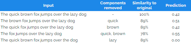
As shown in the table, removing the word “lazy” decreased the predicted negative score to zero, while all other perturbations had a negligible effect on the predictions made by the model. The idea is to fit an interpretable model (such as a decision tree or a linear regression) on the perturbed data set to understand which components influence the original predicted score most. The column “Similarity to original” is the share of words from the initial observation included in the perturbation and is used as weights to fit the simple model.

This example shows the procedure for an NLP model. In the case of tabular data, the perturbed data set is generated by slightly changing input vector values. In the case of images, chunks of the image (called “contiguous pixels”) are grayed out, and predictions are made on the remaining pixels.

As you may have noticed, following this procedure explains why the model made its prediction around the original set of inputs. In layman’s terms, this means that the explanation is valid for a single observation (i.e., a local explanation) and not for all possible observations (i.e., a global explanation).It is for this reason that the explanations made by LIME are considered to be local.

LIME in Python

We will now use LIME to explain the vaderSentiment model. First, install and import both modules:
 

# Install dependencies
!pip install lime
!pip install vaderSentiment

# Import vader model and LIME for text
from vaderSentiment.vaderSentiment import SentimentIntensityAnalyzer
from lime.lime_text import LimeTextExplainer

# Import numpy for formatting
import numpy as np

For each text, Vader returns a dictionary with the text’s negative, positive, neutral and compound scores. Although LIME is model-agnostic (i.e., it will work on any model), it requires the model to be similar in structure to a sklearn object. In particular, the model needs to have a predict_proba method, so we will first modify Vader to make it resemble an sklearn instance.

NOTE: You can skip this step if your model already has a vectorized predict_proba method!
 

# Declare a function that can score multiple texts
def predict_proba(self, texts):

   # Initialize empty list
   ret = []

   # Iterate over texts
   for text in texts:

       # Get negative score
       neg = self.polarity_scores(text).get('neg')

       # Return two outputs: (neg) and (1 - neg)
       ret.append([neg, 1 - neg])

       # Return an array of predictions
       return np.array(ret)

# Add the function to the class as a new method
SentimentIntensityAnalyzer.predict_proba = predict_proba

# Instantiate model
vader = SentimentIntensityAnalyzer()

Let’s now make a prediction on the following text:
I HATE Mondays! I missed the bus and forgot my lunch…

# Declare text
my_angry_text = 'I HATE Mondays! I missed the bus and forgot my lunch...'

# Instantiate explainer (class_names makes the result look nicer)
explainer = LimeTextExplainer(
   class_names=[
       'negative',
       'not-negative'
   ]
)

# Create explanation for text
explanation = explainer.explain_instance(
   My_angry_text,
   Vader.predict_proba,
   num_features=4
)

If you’re in a notebook environment use explanation.show_in_notebook(). Otherwise, use explanation.as_pyplot_figure(). This is what the results look like in a Google Colab notebook:

# Display explanation results
explanation.show_in_notebook()

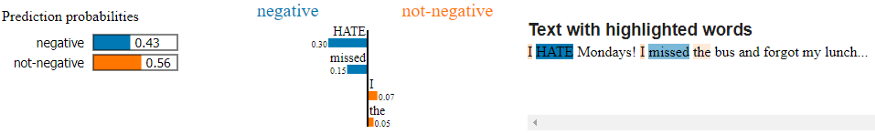
Based on this output, you can tell the word that most influences the text’s negative score is HATE, followed by missed. The words that most heavily influence the text’s non-negative score are I and the.

What is SHAP?

SHAP was proposed in 2017 by Lundberg and Sun-In. Like LIME, it yields local explanations for predictions made by black-box models. The main difference is that SHAP uses game theory (a branch of Economics) to make local explanations.

SHAP stands for SHapley Additive exPlanations and is based on adding Shapley values together (Shapley values are solutions to cooperative games introduced by Lloyd Shapley in 1951). In short, a Shapley value represents the expected value of one player's contribution in a game. To link game theory with machine learning, we must think of the model as the rules of the game and features as players that can either join the fun (i.e., the feature can be observed) or choose not to join (i.e., the feature cannot be observed).

To compute SHAP values, we need:

1. A model we can probe as many times as we need to;
2. A sample of observations; and
3. A very specific structure for the model (to be compatible with SHAP).

NOTE: With LIME, we needed one observation to generate an explanation. Because of how Shapley values are calculated, we will need a whole sample to explain a single observation using SHAP.

Suppose we have a fitted model f that uses input variables X = (X1, X2, …, Xp) to make a prediction, f(X). The goal of SHAP is to explain prediction f(X = x) by measuring how much each feature contributed to the model’s output at X = x.

SHAP in Python (linear regression example)

Calculating Shapley values is a messy process (it requires evaluating the model under many different combinations of input variables). Still, they are easy to visualize when dealing with an additive model (such as linear regression). For the sake of this introduction, imagine we are trying to find the most important variables of a linear regression model that predicts the severity of a patient’s diabetes one year after they were diagnosed.
 
We start by installing SHAP and importing all the dependencies we need to fit a linear regression to the diabetes data set.
 

# Install shap
!pip install shap

# Import dependencies
import shap
import pandas as pd
from sklearn.datasets import load_diabetes
from sklearn.linear_model import LinearRegression

Then, we fit a linear regression model to the data.

# Load features as pandas dataframe
X = pd.DataFrame(

   data=load_diabetes()['data'],
   columns=load_diabetes()['feature_names']
)

# Load target
y = load_diabetes()['target']

# Instantiate model
model = LinearRegression()

# Fit model to data
model.fit(X=X, y=y)

We will now draw a sample from the data (200 observations) to create a partial dependence plot for the Body Mass Index (BMI or also bmi for this article) feature. This step will help us visualize what Shapley values are and where they come from.

# Draw sample of 200 observations
sample = shap.utils.sample(X=X, nsamples=200)

# Partial dependence plot for body-mass index variable
shap.partial_dependence_plot(

   ind='bmi',
   model=model.predict,
   data=sample,
   ice=False,
   model_expected_value=True,
   feature_expected_value=True
)

The vertical red line represents the difference between E[f(x) | bmi = 0.015] and the unconditional expected value E[f(x)]. This is the SHAP value for bmi when bmi = 0.015. Once we have calculated the SHAP values of all the remaining features, we can use the value represented by the red line to understand the importance of bmi in the 42nd observation.

We can explain the importance of each feature for the prediction made on the 42nd observation using a waterfall plot.

# Generate a waterfall plot to explain 42nd obervation
shap.plots.waterfall(shap_values[idx])

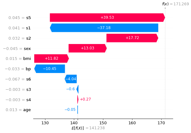
The above plot is read from the bottom up. The x-axis represents the predicted values for the target (the severity of the patient’s diabetes), and the y-axis represents each feature. We start at the unconditional expected value of the predictions made by the model in the sample (141.2). Each horizontal bar represents the SHAP value of each feature, sorted by magnitude in ascending order. This means that the least important feature for the 42nd prediction is age, followed by s4, followed by s3, and so on. Notably, the most important feature is s5, and it had a positive impact on the predicted severity of the patient’s disease. In this example, s5 represents the patient's serum triglycerides level, which is known to increase the risk of strokes and heart disease.

As stated before, the plot starts at E[f(X)]. Note that the plot ends at f(x) = 171.3, the predicted value for the 42nd observation!

# Predict on 42nd observation
print(model.predict(sample.iloc[[idx], :]))

> array([171.26913027])

The fact that the waterfall plot starts at E[f(X)] and ends at E[f(x)] is not a coincidence. Rather, SHAP values are additive, and they always sum up to the difference between the prediction made on the observation we are trying to explain (E[f(x)]) and the unconditional expected value (E[f(X)]) (4). This is a desirable property because it allows us to interpret the sum of all SHAP values as the difference between the prediction when no features are present and the prediction when all features are present. In this context, each feature’s SHAP value represents its contribution toward the prediction made by the model.

Generally speaking, SHAP values cannot be seen in partial dependence plots when we are using nonlinear models (like neural networks). However, the intuition remains the same regardless of what model we are using: we explain the prediction made on a single observation by calculating the SHAP values of all features.