Since the advent of artificial neural networks, solving a specific task for a system based on the neural network has been a problem. This learning task is a rather labor-intensive process, regardless of the size of the input task and the number of neurons in the network. To be successful, you need to prepare the data sets, calculate the deviations from the exact solutions, and select the weight coefficients for each of the neurons. 

If a trained neural network copes quite easily and quickly with the task in the presence of weighted coefficients, then the learning process itself can be thousands or hundreds of thousands of times slower. Such is the nature of neural networks, and the latest mathematical methods and the most powerful computing systems are involved in their training.

Table of contents:

1. Why neural networks are important.
2. Types of neural network training.
3. Mathematical methods used for training.
4. Hardware platforms for neural networks training.
5. Cloud platforms for neural networks training.
6. Conclusion.

Why neural networks are important

Neural networks are successfully used in various fields: business, medicine, technology, geology, and physics. Neural networks have come into practice wherever it is necessary to solve the problems of forecasting, classification, or control. Such impressive success is based on several factors: 

• Wide opportunities. Neural networks are an exceptionally powerful modeling method that can reproduce extremely complex dependencies. In particular, neural networks are non-linear in nature. For many years, linear modeling has been the main modeling method in most areas, since optimization procedures are well developed for it. In problems where the linear approximation is unsatisfactory, however, linear models do not work well. In addition, neural networks cope with the “curse of dimension”, which does not allow modeling linear dependencies in the case of a large number of variables
• Easy to use. Neural networks learn from examples. A neural network user selects representative data and then runs a learning algorithm that automatically perceives the data structure. The user, of course, must have some kind of heuristic knowledge of how to select and prepare data, select the desired network architecture and interpret the results. However, the level of knowledge necessary for the successful use of neural networks is much more modest than, for example, using traditional statistical methods.

Types of neural network training

An artificial neural network is usually trained with a teacher, i.e. supervised methods. This means that there is a training set (dataset) that contains examples with true values: tags, classes, indicators.

Unallocated sets are also used for training neural networks, and appropriate unsupervised methods have been developed for this.

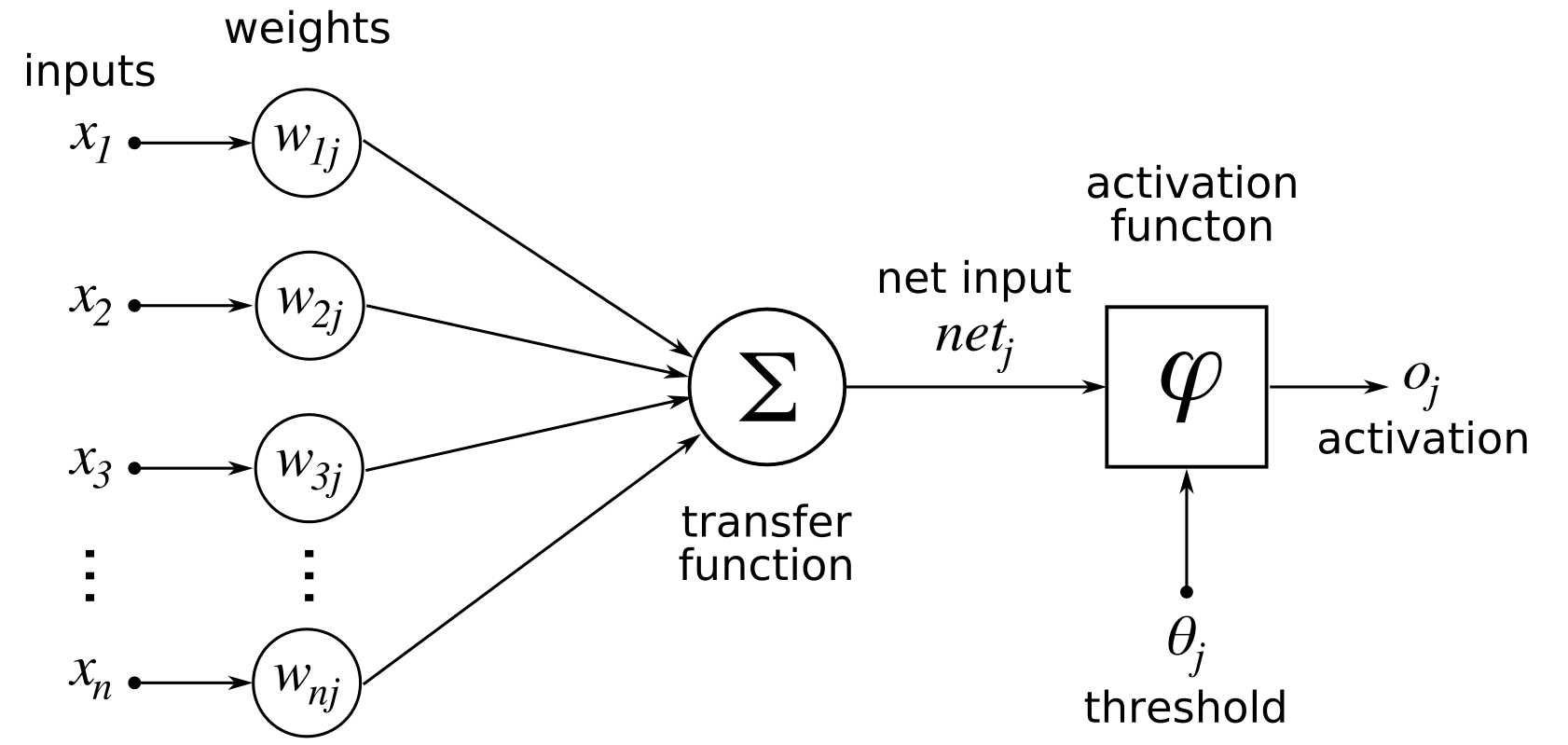
An artificial neural network consists of three components: an Input layer, Hidden (computational) layers, and an Output layer.

Training consists of the selection of coefficients for each neuron in the layers so that with certain input signals we get the necessary set of output signals.

Neural networks are trained in two stages: forward error propagation and reverse error propagation.

Learning methods in a neural network are based on changing weights for each neuron to achieve necessary output parameters with given inputs. These methods minimize the error layer by layer in the neural network.

During forward error propagation, a prediction of the response is made. For instance, for neural networks with two inputs, three neurons, and one output, we can set the initial weights at random: w1, w2. Multiply the input by the weights to form a hidden layer:

h1 = (x1 * w1) + (x2 * w1)
h2 = (x1 * w2) + (x2 * w2)
h3 = (x1 * w3) + (x2 * w3)

The output from the hidden layer is transmitted through a non-linear function (activation function), to obtain the network output:

y = f (h1, h2, h3)

With backpropagation, the error between the actual response and the predicted response is minimized.

Fig. 1. Backpropagation for a simple neural network. 
Image source

Backpropagation efficiently computes the gradient of the loss function with respect to the weights of the network for a single input-output example. This makes it possible to use gradient methods for training multi-layer networks, updating weights to minimize loss. Gradient descent or variants such as stochastic gradient descent are commonly used.

min (loss_value = (y)2 - (y’)2)

The total error is calculated as the difference between the expected value of y (from the training set) and the obtained value of y’ (calculated at the stage of direct propagation of the error) passing through the cost function. The partial derivative of the error is calculated for each weight (these partial differentials reflect the contribution of each weight to the total loss.

Then these differentials are multiplied by a number called the learning rate (η). The result is then subtracted from the corresponding weights. The result is the following updated weights:

w1 = w1 - (η * ∂ (loss-value) / ∂ (w1))
w2 = w2 - (η * ∂ (loss-value) / ∂ (w2))
w3 = w3 - (η * ∂ (loss-value) / ∂ (w3))

The fact that we assume and initialize the weights in a random way, and they give accurate answers, does not sound quite reasonable; however, it works well. 

The choice of the starting point for complex neural network architectures is a rather difficult task, but for most cases, there are proven technologies for choosing the initial approximation. 

In addition, network training is currently not conducted on the entire data set, but on samples of a certain size, the so-called batches. This means that weights in neural networks are tuned from epoch to epoch, to produce better results.

Mathematical methods used for training

Which method is used to train a neural network? Let’s start with a simple and reliable method called gradient descent and then consider the stochastic gradient method.

The process of training a neural net is quite time-consuming. To make this process more efficient, some mathematical ways minimize the number of necessary steps.

Gradient Descent

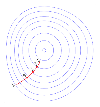
Gradient descent is a first-order iterative optimization algorithm for finding the minimum of a function. To find a local minimum of a function using gradient descent, one takes steps proportional to the negative of the gradient (or approximate gradient) of the function at the current point. If instead, one takes steps proportional to the positive of the gradient, one approaches a local maximum of that function, and the procedure is then known as gradient ascent.

Fig. 2. Gradient Descent. A trajectory goes to the minimum of the loss function

Stochastic Gradient Descent

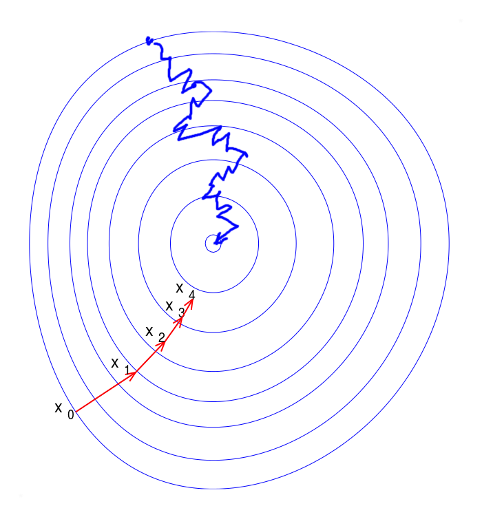
The standard method for training neural networks is the method of stochastic gradient descent (SGD). The problem of gradient descent is that in order to determine a new approximation of the weight vector, it is necessary to calculate the gradient from each sample element, which can greatly slow down the algorithm. The idea of accelerating the stochastic gradient descent algorithm is to use only one element, or some subsample, to calculate the new approximation of the weights.

Neural networks are often trained stochastically; that is, different pieces of data are used at different iterations. This is for at least two reasons. Firstly, the data sets used for training are often too large to store them completely in RAM and/or perform calculations efficiently. Secondly, the optimized function is usually non-convex, so using different parts of the data at each iteration can help to get the model stuck at a local minimum. 

Fig. 3. Stochastic gradient descent (blue). A trajectory is not straight but allows training neural networks on part of the data.

In addition, training of neural networks is usually done with first-order gradient methods, since due to the large number of parameters in the neural network, it is impossible to effectively apply higher-order methods.  

However, it can diverge or converge very slowly if the learning step is not tuned accurately enough. Therefore, there are many alternative methods to accelerate the convergence of learning and save the user from the need to carefully configure hyperparameters. These methods often calculate gradients more efficiently and adaptively change the iteration step.

Other training methods

Other methods of training neural networks (or solving optimization task) sometimes give a better result compared  to classical gradient-based methods:

• Random search method. In the case of simple objective functions, random search methods are less effective than any regular procedure, but they turn out to be useful in more complex cases when the objective function is so complex that it is impossible to establish in advance any of its properties that allow rational selection of search directions. Such random search methods are suitable for any objective function, regardless of whether it is unimodal or not. It is known that for any regular algorithm it is possible to construct a special function (class of functions) on which it will not work. Random search allows you to optimize any function, albeit with different (sometimes very low) efficiency. Random search methods create suitable prerequisites for further application of other search methods. Therefore, they (SP methods) are often used in combination with one or more methods of other types.
• Uniform search method (brute force). The brute force method (uniform search method, brute force search) is the simplest of the methods for finding the values of truly-valued functions by any of the comparison criteria (to maximum, minimum, to a certain constant). As applied to extreme problems, it is an example of a direct method of conditional one-dimensional passive optimization.
• Basin hopping method. Basinhopping is a two-phase method that combines a global stepping algorithm with local minimization at each step. Designed to mimic the natural process of energy minimization of clusters of atoms, it works well for similar problems with “funnel-like, but rugged” energy landscapes.
• Krylov method. Krylov subspace methods work by forming a basis of the sequence of successive matrix powers times the initial residual (the Krylov sequence). The approximations to the solution are then formed by minimizing the residual over the subspace formed. The prototypical method in this class is the conjugate gradient method (CG) which assumes that the system matrix A is symmetric positive-definite. For a symmetric (and possibly indefinite) matrix A one works with the minimal residual method (MINRES). In the case of not even symmetric matrices methods, such as the generalized minimal residual method (GMRES) and the biconjugate gradient method (BiCG), have been derived.
• Adam method. Diederik P. Kingma, Jimmy Ba published this method in 2015: “The method is straightforward to implement, is computationally efficient, has little memory requirements, is invariant to the diagonal rescaling of the gradients, and is well suited for problems that are large in terms of data and/or parameters. The method is also appropriate for non-stationary objectives and problems with very noisy and/or sparse gradients. The hyper-parameters have intuitive interpretations and typically require little tuning.” Adam is an adaptive moment estimation, another optimization algorithm. It combines the idea of the accumulation of motion and the idea of a weaker updating of the scales for typical signs.

It is also necessary to note that you currently do not need to write a learning algorithm from scratch. Popular frameworks like Tensorflow, Teano, Keras, Caffee, etc. now provide high-quality and well-tested tools for training neural networks. 

These tools are implemented on the GPU and parallel computing and save time when you build and train your neural network. Of course, there may be a need to write your own network training algorithm, but this is very rare and for the main network architectures these algorithms are well implemented, described in tutorials and well studied on large sets of input data. 

Do not write your gradient descent from scratch, except for special requirements when the standard method does not suit your neural network.

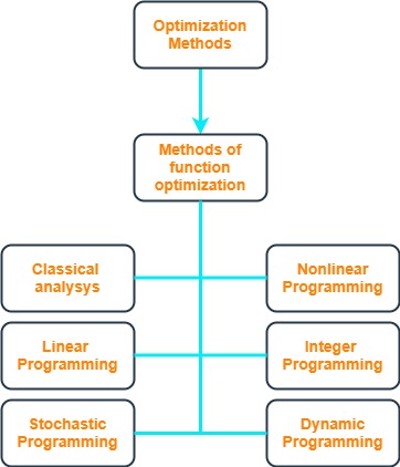
Fig. 4. Diagram of optimization methods for training neural networks.

Hardware platforms for neural networks training

So, we have already decided how to train neural networks, now let's look at what hardware platforms can be used for training. This is an important factor, given that modern requirements for tasks on neural networks require processing dimensions of tens and hundreds of thousands of neurons.

Multi-core processors. Modern general-purpose processors now have sufficiently developed means for organizing high-performance computing due to the presence of several cores and multithreading. This approach is somewhat inferior to specialized hardware solutions for neural networks, but in practice, it can be used to train neural networks.

GPU. Videoboards or Graphical Processor Unit originally developed for 3D graphics applications including games. They have many specialized processor units to calculate math operations in parallel and high-speed memory to store the results. Then NVIDIA created a library called CUDA and it made possible processing general computations on a GPU. This fact allows the increasing speed of training neural networks thousand and thousand times compared to regular CPU.

TPU. To make a more efficient processor for neural networks, Google developed a Tensor processing unit (TPU). Google released its first TPU in 2016. And now TensorFlow Python APIs and graph operators are available on Cloud TPU. The TPUs do not need as much mathematical precision for training neural networks, i.e. it needs fewer resources to make a huge number of calculations.

FPGA. Reconfigurable devices such as field-programmable gate arrays (FPGA) make it easier to evolve hardware, frameworks, and software for building effective neural network systems. According to some sources, Intel acquired Altera to use FPGAs to accelerate AI in order to integrate them into server CPUs. The advantage of this approach is that it gives high performance and allows you to change the architecture of the neural network for a specific task.

Special processors. Many companies are now working on creating effective solutions for training neural networks using specialized processors. This makes it possible to realize the necessary computing power for a certain class of tasks of neural processors, such as voice recognition, auto control, image, and video recognition. With less power consumption, such specialized solutions will give better results compared to GPU and TPU, and these solutions are compact for placement in a small form factor. (NVIDIA Jetson Xavier NX, Intel Movidius Myriad 2, Mobileye EyeQ, IBM TrueNorth — neuromorphic processor, Cambricon MLU100, Cerebras Wafer Scale Engine (WSE) )

Cloud platforms for neural networks training

After considering neural network training algorithms, let's look at how we can speed up this process. One possible way is to use a GPU on-premises. Another effective way is to use cloud computing.

As in all modern IT industries, training of neural networks can now be carried out in cloud systems. At the same time, you are given the opportunity to use modern frameworks such as TensorFlow, Theano, Caffee, etc. and run training on GPU or TPU. 

Especially important to mention are such cloud systems as Amazon EC2 (P2, P3, G3) instances, Intel Nervana Cloud, Google Collaboratory, Azure NVv4, and IBM Watson Neural Network Modeler.

And why do we need to run the training of neural networks in the cloud? After all, you can do this on your computer or server, right? But if you need to train your neural network quite intensively, then you need to deploy a couple of servers with a high-performance and expensive GPU.  How can this be done quickly and inside of a tight budget? 

The cloud system allows you to get access to just such a configuration and a hardware platform that is inexpensive and as fast as possible and allows scaling both up and down. You pay only for that resource when you train a neural network. This approach is very beneficial for the budget.

Conclusion

To summarize the above, in modern conditions, the training of your neural network will already be much faster than was previously possible. In addition, this is a rather interesting process when you experiment with various training methods, correctly build the input data and find the right starting point for the training parameters of the neural network. 

Use high-performance hardware platforms, train your neural networks in cloud systems, use the best mathematical methods that are implemented in the most modern frameworks. And good luck to you in building successful systems based on neural networks.